本文介绍怎么使用Python库PuLP来解决一些线性规划和线性整数规划问题,本文主要翻译了Ben Alex Keen的博客、官方文档数独示例。包括了工厂调度、资源分配和数独等问题的示例。
目录
概述
线性规划(Linear Programming),有时候也叫线性优化,它是在线性等式或者不等式的约束下解决最大化或者最小化一个线性的目标函数的问题。Leonard Kantrovich因为使用线性规划解决了最优的资源分配问题而获得了1975年的诺贝尔经济学奖。
后面我们会使用线性规划来解决如下问题:
- 调度 - 调度工厂的生成方案来最小化成本
- 资源分配 - 怎么分配资源以最大化利润
- 混合问题 - 怎么低成本的混合食品的成分
- 数独
本文除了一节简单的线性规划基本概念介绍外大部分篇幅都是通过示例来介绍怎么来解决实际问题。这里会使用Python和PuLP库来解决线性规划问题。PuLP使用Python简洁的语法来定义问题,并且内置了CBC求解器(Solver);除了内置的求解器,PuLP也很容易集成各种开源或者商业的线性规划求解器。
线性规划简介
本节介绍怎么通过绘图”手动”对线性优化问题求解。假设我们需要优化的目标(线性)函数为:
\[Z = 4x+3y\]我们希望最大化Z,x和y是决策变量,并且需要满足如下的线性约束:
\[\begin{split} x & \geq 0 \\ y & \geq 2 \\ 2y & \leq 25 – x \\ 4y & \geq 2x – 8 \\ y & \leq 2x -5 \\ \end{split}\]下面我们绘制上面约束条件的可行域:
import numpy as np
import matplotlib.pyplot as plt

# Construct lines
# x > 0
x = np.linspace(0, 20, 2000)
# y >= 2
y1 = (x*0) + 2
# 2y <= 25 - x
y2 = (25-x)/2.0
# 4y >= 2x - 8
y3 = (2*x-8)/4.0
# y <= 2x - 5
y4 = 2 * x -5

# Make plot
plt.plot(x, y1, label=r'$y\geq2$')
plt.plot(x, y2, label=r'$2y\leq25-x$')
plt.plot(x, y3, label=r'$4y\geq 2x - 8$')
plt.plot(x, y4, label=r'$y\leq 2x-5$')
plt.xlim((0, 16))
plt.ylim((0, 11))
plt.xlabel(r'$x$')
plt.ylabel(r'$y$')

# Fill feasible region
y5 = np.minimum(y2, y4)
y6 = np.maximum(y1, y3)
plt.fill_between(x, y5, y6, where=y5>y6, color='grey', alpha=0.5)
plt.legend(bbox_to_anchor=(1.05, 1), loc=2, borderaxespad=0.)

plt.show()
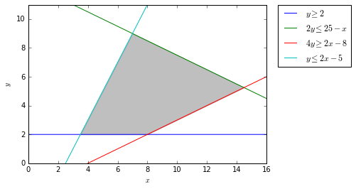 图:可行域
图:可行域
绘制出来的可行域如上图所示,读者可以对照图例(legend)的颜色辨识这4条直线。如果存在最优解的话,那么显然最优解是在这四条直线围成的区域里。我们不做证明,如果存在最优解,则可行域的顶点一定是最优解。在这个例子里,可行域只有4个顶点,因此我们需要检查这4个点哪个是最优解。
我们要最大化的是$Z = 4x + 3y$。
首先是$y = 2 \text{ and } 4y = 2x – 8$的交点:
\[y \geq 2 \text{ and } 4y \geq 2x – 8 \\ 2 = \dfrac{2x – 8}{4} \\ x = 8 \\ y = 2 \\ Z = (4 \times 8 + 3 \times 2) = 38 \\\]第二个:
\[2y \leq 25 – x \text{ and } y \leq 2x – 5 \\ \dfrac{25 – x}{2} = 2x – 5 \\ x = 7 \\ y = 9 \\ Z = (4 \times 7 + 3 \times 9) = 55 \\\]第三个:
\[2y \leq 25 – x \text{ and } 4y \geq 2x – 8 \\ \dfrac{25 – x}{2} = \dfrac{2x – 8}{4} \\ x = 14.5 \\ y = 5.25 \\ Z = (4 \times 14.5 + 3 \times 5.25) = 73.75 \\\]第四个:
\[y \geq 2 \text{ and } y \leq 2x – 5 \\ 2 = 2x-5 \\ x = 3.5 \\ y = 2 \\ Z = (4 \times 3.5 + 3 \times 2) = 20\]这个四个顶点里Z的最大值是73.75,其中x是14.5,y是5.25。
上面的方法只适合于变量很少和约束的情况,比如平面的4条直线两两相交理论上最多有$\tbinom{4}{2}=6$。根据图形我们只检查了上面4组直线的交点,但是高维的空间怎么画?一般可以使用单纯形法或者内点法求解,我们这里不做介绍,感兴趣的读者可以搜索线性规划(优化)的书籍。
PuLP简介
PuLP是一个开源的线性规划包(实际还包括整数规划)。可以使用pip来安装,具体参考这里。
在这一节,我们用PuLP来求解前面的那个简单线性规划问题:
我们需要最大化的目标函数是:
\[Z = 4x + 3y\]约束条件是:
\[x \geq 0 \\ y \geq 2 \\ 2y \leq 25 – x \\ 4y \geq 2x – 8 \\ y \leq 2x -5 \\\]我们首先导入PuLP:
import pulp
接着我们初始化一个问题类,把它命名为”My_LP_problem”。因为我们的目标是最大化一个线性函数,所以需要传给它一个常量LpMaximize:
my_lp_problem = pulp.LpProblem("My_LP_Problem", pulp.LpMaximize)
然后我们定义连续的决策变量,其中x的下界是0$(x \ge 0)$,y的下界是2。
x = pulp.LpVariable('x', lowBound=0, cat='Continuous')
y = pulp.LpVariable('y', lowBound=2, cat='Continuous')
然后我们定义目标函数和约束条件,PuLP重载符号+=用于这个目的,我们首先定义目标函数:
# 目标函数,命名为Z
my_lp_problem += 4 * x + 3 * y, "Z"
接下来是约束条件:
# Constraints
my_lp_problem += 2 * y <= 25 - x
my_lp_problem += 4 * y >= 2 * x - 8
my_lp_problem += y <= 2 * x - 5
细心的读者可能会问:为什么前面是4个约束条件(其实是5个),这里变成了3个?因为我们把一个约束条件直接放到决策变量的下界里了,我们完全可以这样:
# 不定义下界,默认的下界是负无穷
y = pulp.LpVariable('y', cat='Continuous')
my_lp_problem += y >= 2
但是用前面的方法更加简单高效。下面我们打印my_lp_problem出来看看:
print(my_lp_problem)
输出结果为:
My_LP_Problem:
MAXIMIZE
4*x + 3*y + 0
SUBJECT TO
_C1: x + 2 y <= 25

_C2: - 2 x + 4 y >= -8

_C3: - 2 x + y <= -5

VARIABLES
x Continuous
2 <= y Continuous
PuLP支持很多开源的线性规划求解器(solver),比如CBC和GLPK;此外它也支持商业(收费)的求解器比如Gurobi和IBM的CPLEX。
默认的是CBC,安装PuLP是默认就会安装。对于大部分问题来说,来自COIN-OR的CBC开源求解器就够用了。
下面我们来求解:
my_lp_problem.solve()
print(pulp.LpStatus[my_lp_problem.status])
输出的结果是’Optimal’,说明找到了最优解。my_lp_problem.status是一个常量,pulp.LpStatus是一个dict,把常量变成可读的字符串:
LpStatus = {
    LpStatusNotSolved:"Not Solved",
    LpStatusOptimal:"Optimal",
    LpStatusInfeasible:"Infeasible",
    LpStatusUnbounded:"Unbounded",
    LpStatusUndefined:"Undefined",
    }
这些常量的含义是:
- Not Solved
- 还没有调研solve()函数前的状态。
- Optimal
- 找到了最优解。
- Infeasible
- 问题没有可行解(比如定义了constraints x <= 1并且x >=2这样的约束)。
- Unbounded
- 约束条件是无界的(not bounded),最大化会导致无穷大(比如只有一个x >= 3这样的约束)。
- Undefined
- 最优解可能存在但是没有求解出来。
解出来之后我们可以看最优解以及目标函数的最优值:
for variable in my_lp_problem.variables():
    print("{} = {}".format(variable.name, variable.varValue))

print(pulp.value(my_lp_problem.objective))
输出结果是:
x = 14.5
y = 5.25
73.75
这和我们前面通过作图手动求解的结果是一样的。这个例子完整的代码在这里。
通过这个简单的例子了解了PuLP的用法后我们下面来解决一些更加实际的问题。
资源分配问题
假设我们给一家生产豪车的厂商做优化,厂商可以生产两种车A和B。它们以一个月(30)作为一个周期来优化我们的利润。厂商有一个机器人,2个工程师和一个推销员。机器人和工程师都不休息(这是血汗工厂),但是推销员只工作21天(工程师最没地位)。生产和销售一辆车需要不同的机器人、工程师和推销员的工时:生产和销售一辆A车需要3天的机器人工时、5天的工程师工时和1.5天的推销员工时;而B需要4天的机器人工时、6天的工程师工时和3天的推销员工时。A车的利润是€30,000,而B车是€45,000。目前的方案是每辆车生产和销售4辆,利润是€300,000,现在我们需要找到利润更高的方案。我们下面把它建模成一个线性规划问题,决策变量A和B代表两种车的产量。那么我们优化的目标函数是:
\[Profit=30,000A+45,000B\]约束条件是:
\[A \geq 0 \\ B \geq 0 \\ 3A + 4B \leq 30 \\ 5A + 6B \leq 60 \\ 1.5A + 3B \leq 21 \\\]下面我们用PuLP来求解:
import pulp
# Instantiate our problem class
model = pulp.LpProblem("Profit_maximising_problem", pulp.LpMaximize)
和前面不同,我们现在的决策变量是离散的而不是连续的变量,因为我们不能生产半辆车出去卖,所以cat是’Integer’:
A = pulp.LpVariable('A', lowBound=0, cat='Integer')
B = pulp.LpVariable('B', lowBound=0, cat='Integer')
然后定义目标函数和约束:
# Objective function
model += 30000 * A + 45000 * B, "Profit"

# Constraints
model += 3 * A + 4 * B <= 30
model += 5 * A + 6 * B <= 60
model += 1.5 * A + 3 * B <= 21
最后是求解和输出最优方案:
# Solve our problem
model.solve()
print(pulp.LpStatus[model.status])

# Print our decision variable values
print("Production of Car A = {}".format(A.varValue))
print("Production of Car B = {}".format(B.varValue))
结果为:
Optimal
Production of Car A = 2.0
Production of Car B = 6.0
330000.0
最优的方案是生成2两辆A和6辆B,利润是€330,000,比如之前的利润提升了10%,老板应该很高兴我们给出的方案。本节的代码在这里。
混合问题
我们假设有如下3种原料猪肉、小麦和淀粉,它们各自的价格和数量如下表:
| 原料 | 成本 (€/kg) | 数量 (kg) |
|---|---|---|
| 猪肉 | 4.32 | 30 |
| 小麦 | 2.46 | 20 |
| 淀粉 | 1.86 | 17 |
我们可以用这些原料制作两种烤肠:
- 便宜的(猪肉含量>40%)
- 贵的(猪肉含量>60%)
每根香肠重量为50克(0.05 kg)。政府部门规定淀粉的含量不能超过25%。另外我们和一个屠宰场签定了合约,至少要购买23kg的猪肉。我们的客户向我们订购了350个便宜的烤肠和500个贵的烤肠,现在我们需要设计这两种烤肠里3种原料的比例,目标是用最少的成本。下面我们把这个问题用数学语言来描述(也就是建模),首先是定义决策变量:
\[p_e = \text{便宜的(economy)烤肠中猪肉(pork)的总含量,单位kg} \\ w_e = \text{便宜的(economy)烤肠中小麦(wheat)的总含量,单位kg} \\ s_e = \text{便宜的(economy)烤肠中淀粉(starch)的总含量,单位kg} \\ p_p = \text{贵的(premium)烤肠中猪肉(pork)的总含量,单位kg} \\ w_p = \text{贵的(premium)烤肠中小麦(wheat)的总含量,单位kg} \\ s_p = \text{贵的(premium)烤肠中淀粉(starch)的总含量,单位kg} \\\]约束条件是:
\[p_e + w_e + s_e = 350 \times 0.05 \\ p_p + w_p + s_p = 500 \times 0.05 \\ p_e \geq 0.4(p_e + w_e + s_e) \\ p_p \geq 0.6(p_p + w_p + s_p) \\ s_e \leq 0.25(p_e + w_e + s_e) \\ s_p \leq 0.25(p_p + w_p + s_p) \\ p_e + p_p \leq 30 \\ w_e + w_p \leq 20 \\ s_e + s_p \leq 17 \\ p_e + p_p \geq 23 \\\]下面用PuLP来解决这个问题。首先还是导入包和构造LpProblem:
import pulp
# Instantiate our problem class
model = pulp.LpProblem("Cost_minimising_blending_problem", pulp.LpMinimize)
我们这里有6个决策变量,当然我们还是可以一个一个的定义这些变量。但是随着问题变复杂,我们的决策变量可能成百上千,一个个定义得累死。不过通常这些变量可以分为类似的组,我们可以一次定义一组变量。LpVariable提供了dicts函数来解放我们的工作:
# Construct our decision variable lists
sausage_types = ['economy', 'premium']
ingredients = ['pork', 'wheat', 'starch']

ing_weight = pulp.LpVariable.dicts("weight kg",
                                     ((i, j) for i in sausage_types for j in ingredients),
                                     lowBound=0,
                                     cat='Continuous')
pulp.LpVariable.dicts的第二个参数是这一组变量的名字,我们这里用tuple来表示,比如(‘economy’,’pork’)就表示前面的$p_e$。我们用生成器来生成这些名字tuple,也就是:
gen = ((i, j) for i in sausage_types for j in ingredients)
for (i, j) in gen:
    print("i={}, j={}".format(i,j))
print(gen)
先定义目标函数:
# Objective Function
model += (
    pulp.lpSum([
        4.32 * ing_weight[(i, 'pork')]
        + 2.46 * ing_weight[(i, 'wheat')]
        + 1.86 * ing_weight[(i, 'starch')]
        for i in sausage_types])
)
接下来是定义约束:
# 约束
# 350个便宜的和500个贵的烤肠,每个0.05 kg
model += pulp.lpSum([ing_weight['economy', j] for j in ingredients]) == 350 * 0.05
model += pulp.lpSum([ing_weight['premium', j] for j in ingredients]) == 500 * 0.05

# 便宜的烤肠猪肉占比大于pork,贵的大于60%,
# 其实pulp.lpSum([ing_weight['economy', j] for j in ingredients]) == 350 * 0.05
# 改成350 * 0.05更简单
model += ing_weight['economy', 'pork'] >= (
    0.4 * pulp.lpSum([ing_weight['economy', j] for j in ingredients]))

model += ing_weight['premium', 'pork'] >= (
    0.6 * pulp.lpSum([ing_weight['premium', j] for j in ingredients]))

# 淀粉比率小于25%
model += ing_weight['economy', 'starch'] <= (
    0.25 * pulp.lpSum([ing_weight['economy', j] for j in ingredients]))

model += ing_weight['premium', 'starch'] <= (
    0.25 * pulp.lpSum([ing_weight['premium', j] for j in ingredients]))

# 我们最多用30kg猪肉,20kg小麦和17kg淀粉
model += pulp.lpSum([ing_weight[i, 'pork'] for i in sausage_types]) <= 30
model += pulp.lpSum([ing_weight[i, 'wheat'] for i in sausage_types]) <= 20
model += pulp.lpSum([ing_weight[i, 'starch'] for i in sausage_types]) <= 17

# 我们已经预定了23kg猪肉,所以一定要用掉
model += pulp.lpSum([ing_weight[i, 'pork'] for i in sausage_types]) >= 23
前面我们用+号来表示线性约束,但是现在我们要对很多个变量进行线性约束,这个时候就需要用到pulp.lpSum函数来简化。比如第一个约束:
\[p_e + w_e + s_e = 350 \times 0.05\]我们当然可以这样来写:
model += [ing_weight['economy', 'pork'] + [ing_weight['economy', 'wheat'] + ing_weight['economy', 'starch'] == 350 * 0.05
如果变量成百上千,那这行代码就上万列了,而且写起来也得累死。我们用lpSum就简单的多:
model += pulp.lpSum([ing_weight['economy', j] for j in ingredients]) == 350 * 0.05
然后就是求解和输出结果:
# Solve our problem
model.solve()
print(pulp.LpStatus[model.status])


for var in ing_weight:
    var_value = ing_weight[var].varValue
    print("The weight of {0} in {1} sausages is {2} kg".format(var[1], var[0], var_value))

total_cost = pulp.value(model.objective)

print("The total cost is €{} for 350 economy sausages and 500 premium sausages".format(round(total_cost, 2)))
输出结果为:
Optimal
The weight of pork in economy sausages is 7.0 kg
The weight of wheat in economy sausages is 6.125 kg
The weight of starch in economy sausages is 4.375 kg
The weight of pork in premium sausages is 16.0 kg
The weight of wheat in premium sausages is 2.75 kg
The weight of starch in premium sausages is 6.25 kg
The total cost is €140.96 for 350 economy sausages and 500 premium sausages
完整的代码点击这里。
使用二值变量解决规划问题
假设我们有两个生产工厂(A和B)以及估计的需求量。我们希望用最小的成本来制定每个工厂的产量来满足客户的需求。每个工厂可以处于如下两种状态:
- 停工
- 也就是不生成任何产品
- 开工
- 生产的产品数量在最小产能和最大产能之间
每个工厂有固定的成本,不开工就没有,但是一旦开工,不管生产多少都需要这么多的成本。另外就是可变的成本,以单位产品的价格来计算。这些成本(固定的和可变的)都是每月变动的。并且我们知道5月份B工厂需要停工整修。下面我们先来看看数据,这些成本数据都保持在一个CSV文件里,我们会使用Pandas库来读取它。
import pandas as pd
import pulp
导入了pandas和pulu之后我们来读取文件:
factories = pd.DataFrame.from_csv('factory_variables.csv', index_col=['Month', 'Factory'])
print(factories)
结果如下表(为了好看,排版成HTML)
| Max_Capacity | Min_Capacity | Variable_Costs | Fixed_Costs | ||
|---|---|---|---|---|---|
| Month | Factory | ||||
| 1 | A | 100000 | 20000 | 10 | 500 |
| B | 50000 | 20000 | 5 | 600 | |
| 2 | A | 110000 | 20000 | 11 | 500 |
| B | 55000 | 20000 | 4 | 600 | |
| 3 | A | 120000 | 20000 | 12 | 500 |
| B | 60000 | 20000 | 3 | 600 | |
| 4 | A | 145000 | 20000 | 9 | 500 |
| B | 100000 | 20000 | 5 | 600 | |
| 5 | A | 160000 | 20000 | 8 | 500 |
| B | 0 | 0 | 0 | 0 | |
| 6 | A | 140000 | 20000 | 8 | 500 |
| B | 70000 | 20000 | 6 | 600 | |
| 7 | A | 155000 | 20000 | 5 | 500 |
| B | 60000 | 20000 | 4 | 600 | |
| 8 | A | 200000 | 20000 | 7 | 500 |
| B | 100000 | 20000 | 6 | 600 | |
| 9 | A | 210000 | 20000 | 9 | 500 |
| B | 100000 | 20000 | 8 | 600 | |
| 10 | A | 197000 | 20000 | 10 | 500 |
| B | 100000 | 20000 | 11 | 600 | |
| 11 | A | 80000 | 20000 | 8 | 500 |
| B | 120000 | 20000 | 10 | 600 | |
| 12 | A | 150000 | 20000 | 8 | 500 |
| B | 150000 | 20000 | 12 | 600 |
下面是每个月的需求,在monthly_demand文件里:
demand = pd.DataFrame.from_csv('monthly_demand.csv', index_col=['Month'])
| Demand | |
|---|---|
| Month | |
| 1 | 120000 |
| 2 | 100000 |
| 3 | 130000 |
| 4 | 130000 |
| 5 | 140000 |
| 6 | 130000 |
| 7 | 150000 |
| 8 | 170000 |
| 9 | 200000 |
| 10 | 190000 |
| 11 | 140000 |
| 12 | 100000 |
我们首先来定义决策变量,首先是A和B两个工程每个月的产量,这是一个整数:
production = pulp.LpVariable.dicts("production",
                                     ((month, factory) for month, factory in factories.index),
                                     lowBound=0,
                                     cat='Integer')
我们还是使用LpVariable.dicts来定义一组变量,这组变量的名字用(month, factory)这个tuple来命名,pandas读取时的”index_col=[‘Month’, ‘Factory’]”就把month和factory作为索引来读取csv文件,我们这里用factories.index就可以得到所有月份和工厂的组合。我们可以把factories看成一个dict,key是(month, factory)这个tuple,value是其它的column,也就是Max_Capacity、Min_Capacity、Variable_Costs和Fixed_Costs。
接下来我们还要定义每个月是否开工这组决策变量,它决定了是否有固定的成本。
factory_status = pulp.LpVariable.dicts("factory_status",
                                     ((month, factory) for month, factory in factories.index),
                                     cat='Binary')
它的名字也是factories.index得到的tuple的list,但是它的类别不是”Integer”而是”Binary”。
有些读者可能会觉得是不是有production就足够了,因为如果production>0就意味着开工。理论上是这样的,但是这种逻辑推理关系是不能在线性规划上使用的,因为PuLP不是逻辑编程语言(后面我们会介绍怎么用”trick”的方法实现简单的逻辑),我们可以简单的在Python写if/else,但是线性规划本身都是一些线性的函数,怎么用线性函数来表示逻辑并不那么容易。事实上我们在后面的约束里能看到factory_status和production是存在约束(逻辑)关系的,比如如果一个工厂在3月份没有开工,那它在3月份的产量必须是0。
在定义约束前不用忘了定义问题和目标函数:
model = pulp.LpProblem("scheduling_problem", pulp.LpMinimize)

model += pulp.lpSum(
    [production[month, factory] * factories.loc[(month, factory), 'Variable_Costs'] for month, factory in factories.index]
    + [factory_status[month, factory] * factories.loc[(month, factory), 'Fixed_Costs'] for month, factory in factories.index]
)
我们的目标函数也就是成本分为两部分,固定的成本和可变的(根据产量)成本。固定的成本就是factory_status乘以Fixed_Costs,因为factory_status=1/0表示开工/停工,所以如果停工就是0,如果开工就是Fixed_Costs。而可变的成本就是production[month, factory]乘以这个工厂这个月的可变成本,可以用factories.loc[(month, factory), ‘Variable_Costs’]得到。如果对pandas不熟的读者可以参考文档。
接下来就是定义约束,首先每个月两个工厂的产量加起来要等于需求:
months = demand.index
for month in months:
    model += production[(month, 'A')] + production[(month, 'B')] == demand.loc[month, 'Demand']
前面我们也说了,用线性约束来表示逻辑约束是需要一些技巧(trick)的。比如我们这个问题里,如果一个工厂不开工,它的产量就必须是0,如果开工,则它的产量必须在最大和最小产能之间。后面我们会介绍怎么表示逻辑约束,这里我们首先给出这个约束,然后理解一下它确实可以实现我们的需求就可以了。
for month, factory in factories.index:
    min_production = factories.loc[(month, factory), 'Min_Capacity']
    max_production = factories.loc[(month, factory), 'Max_Capacity']
    model += production[(month, factory)] >= min_production * factory_status[month, factory]
    model += production[(month, factory)] <= max_production * factory_status[month, factory]
我们来看一下,如果factory_status[month, factory]==0,则增加了如下两个约束:
production[(month, factory)] >= 0
production[(month, factory)] <= 0
因此production[(month, factory)]只能等于0。如果factory_status[month, factory]==1,则增加了如下两个约束:
production[(month, factory)] >= min_production
production[(month, factory)] <= max_production
这正是我们想要的约束,读者可能会说,这有点tricky,我们怎么就能想到用这样的方式来表示逻辑关系,万一一个非常复杂的与或非逻辑表达式给到我,那我怎么用线性约束来表示呢?不用担心,后面我们会介绍。
另外一个约束就是B厂5月份要停工:
model += factory_status[5, 'B'] == 0
model += production[5, 'B'] == 0
其实只需要第一个就行了,但是加上第二个(可能)能够让优化速度快一点,因为不需要它通过不等式来确定factory_status等于0了。
约束定义完了,剩下的就简单了(复杂的部分交给PuLP了):
model.solve()
print(pulp.LpStatus[model.status])
结果是’Optimal’,非常好!下面我们把所有的决策变量打印出来,这就是我们的最优方案:
output = []
for month, factory in production:
    var_output = {
        'Month': month,
        'Factory': factory,
        'Production': production[(month, factory)].varValue,
        'Factory Status': factory_status[(month, factory)].varValue
    }
    output.append(var_output)
output_df = pd.DataFrame.from_records(output).sort_values(['Month', 'Factory'])
output_df.set_index(['Month', 'Factory'], inplace=True)
print(output_df)
为了打印漂亮的表格,我们把决策变量放到pandas的一个DateFrame里,结果为(变成了HTML):
| Factory Status | Production | ||
|---|---|---|---|
| Month | Factory | ||
| 1 | A | 1 | 70000 |
| B | 1 | 50000 | |
| 2 | A | 1 | 45000 |
| B | 1 | 55000 | |
| 3 | A | 1 | 70000 |
| B | 1 | 60000 | |
| 4 | A | 1 | 30000 |
| B | 1 | 100000 | |
| 5 | A | 1 | 140000 |
| B | 0 | 0 | |
| 6 | A | 1 | 60000 |
| B | 1 | 70000 | |
| 7 | A | 1 | 90000 |
| B | 1 | 60000 | |
| 8 | A | 1 | 70000 |
| B | 1 | 100000 | |
| 9 | A | 1 | 100000 |
| B | 1 | 100000 | |
| 10 | A | 1 | 190000 |
| B | 0 | 0 | |
| 11 | A | 1 | 80000 |
| B | 1 | 60000 | |
| 12 | A | 1 | 100000 |
| B | 0 | 0 |
我们发现停工的工程产量确实是0,下面我们看一下最小的成本:
print(pulp.value(model.objective))
结果输出是”12906400.0”。本节的完整源代码在这里。
逻辑约束的表示
前面我们还有一个问题没有解决,那就是怎么用二值变量的线性约束来表示这些二值变量(逻辑变量)的与或非关系。非的关系是很容易实现的,比如假设”x1+x2<=1”表示一种逻辑关系,我们想求非的话只要变成”x1+x2>1”就可以了。注意,PuLP是不支持”>”或者”<”的,只能是”<=”、”>=”或者”==”。那怎么表示”>”或者”<”呢?如果是整数变量的话,可以把”>a”表示成”>=a+1”。如果是非整数变量就只能用非常tricky的加一个非常小的数了:
x1+x2>1 等价于 x1+x2>=1+0.00000001
因此,我们只需要考虑怎么实现两个二值变量的或运算以及非运算。理论上有了两个布尔变量的与或非,其它任意的布尔表达式都可以用而合取范式来表示。不过在介绍两个布尔变量前,我们看看一个布尔变量的情况。
一个布尔变量
首先是最终的值等于这个变量:
if x1 == 1:
    y1 == 1
elif x1 == 0:
    y1 == 0
我们直接用:
y1 == x1
读者可能会奇怪,既然y1等于x1,那么为什么还要定义两个变量,直接定义一个就行了。理论上是可以,但是有些问题定义成两个变量可能更加清晰,它们可能代表不同的含义,只不过有一个约束要求它们的值相同而已。
另外就是相反的情况:
if x1 == 1:
    y1 == 0
elif x1 == 0:
    y1 == 1
可以用下式来表示:
x1 + y1 == 1
我们可以验证一下:如果x1等于1,则y1=1-x1(1)=0;否则如果x1等于0,则y1=1-x1(0)=1。
逻辑与
逻辑与可以用如下的函数来生成与之等价的线性约束的集合:
def make_io_and_constraint(y1, x1, x2, target_x1, target_x2):
    """
    Returns a list of constraints for a linear programming model
    that will constrain y1 to 1 when
    x1 = target_x1 and x2 = target_x2;
    where target_x1 and target_x2 are 1 or 0
    """
    binary = [0,1]
    assert target_x1 in binary
    assert target_x2 in binary

    if target_x1 == 1 and target_x2 == 1:
        return [
            y1 >= x1 + x2 - 1,
            y1 <= x1,
            y1 <= x2
        ]
    elif target_x1 == 1 and target_x2 == 0:
        return [
            y1 >= x1 - x2,
            y1 <= x1,
            y1 <= (1 - x2)
        ]
    elif target_x1 == 0 and target_x2 == 1:
        return [
            y1 >= x2 - x1,
            y1 <= (1 - x1),
            y1 <= x2
        ]
    else:
        return [
            y1 >= - (x1 + x2 -1),
            y1 <= (1 - x1),
            y1 <= (1 - x2)
        ]
看起来有一些复杂,我们来看一个例子。比如我们想实现”y1 == ((x1==1) AND (x2==0))”,那么我们会调用:
make_io_and_constraint(y1, x1, x2, 1, 0)
则执行的路径是:
        return [
            y1 >= x1 - x2,
            y1 <= x1,
            y1 <= (1 - x2)
        ]
我们来验证一下,如果x1=1并且x2=0,则返回的三个约束是:
y1 >= 1 - 0
y1 <= 1
y1 <= (1 - 0)
显然y1=1。如果x1=1并且x2=1,则返回:
y1 >= 1 - 1
y1 <= 1
y1 <= (1 - 1)
求解这三个不等式得到y1=0。类似的另外x1=0的两种情况读者也可以一一验证。
可能有好奇的读者会说要验证这个很容易,但是怎么想到用这样三个不等式就能得到我们需要的”y1 == ((x1==1) AND (x2==0))”?这是个好问题,这个问题的答案很难。就像我们要验证(看懂)一个几何题的证明可能并不困难,但是怎么”想”出来就很难。或者我们还能不能多问一个问题,为什么需要三个线性约束?两个行不行?有的人可能会说这是”灵感”,但是我个人认为”灵感”并不存在,所谓的”灵感”只是搜索后的一种结果。当然这是一个哲学问题,感兴趣的读者可以阅读人工智能能否实现?。我们这里其实可以使用简单的穷举”搜索”法,x1、x2和y1共有3个变量,我们可以用系数(-1、0和1)来列举所有的不等式:
0*y1 >= 0*x1 + 0*y1 + const(-1,0,1)
0*y1 >= 0*x1 + -1 * y1 + const(-1,0,1)
...
这里的不等式个数是有限的,假设为N个,然后我们从N个里挑出3个,这有$\tbinom{N}{3}$种,我们一一验证,直到找到这个:
            y1 >= 1 * x1 + -1 * x2 + 0,
            -1 *y1 >=  -1 * x1 + 0 * x2 + 0,
            -1 * y1 >= 0 * x1 + 1 * x2 + (-1)
化简一下就是前面得到的那三个不等式。当然我知道有些读者还有一下更加”灵感”的方法,但是我觉得那些”灵感”只是用了一下启发式的规则来进行裁剪,或者用了比穷举更好的一下搜索算法,比如动态规划或者贪心算法。
布尔或
def make_io_or_constraint(y1, x1, x2, target_x1, target_x2):
    """
    Returns a list of constraints for a linear programming model
    that will constrain y1 to 1 when
    x1 = target_x1 or x2 = target_x2;
    where target_x1 and target_x2 are 1 or 0
    """
    binary = [0, 1]
    assert target_x1 in binary
    assert target_x2 in binary

    if target_x1 == 1 and target_x2 == 1:
        return [
            y1 <= x1 + x2,
            y1 * 2 >= x1 + x2
        ]
    elif target_x1 == 1 and target_x2 == 0:
        return [
            y1 <= x1 - x2 + 1,
            y1 * 2 >= x1 - x2 + 1
        ]
    elif target_x1 == 0 and target_x2 == 1:
        return [
            y1 * 2 <= 1 - x1 + x2,
            y1 >= -x1 + x2
        ]
    else:
        return [
            y1 * 2 <= 2 - (x1 + x2),
            y1 >= 1 - (x1 + x2)
        ]
和前面类似,读者可以验证这个函数确实实现了或的逻辑。
规划问题的扩展
下面我们扩展一下前面一节的例子,再增加一个启动成本,从而看怎么把上面的函数用起来。前面我们的问题有两类成本:
- 固定成本
- 只要这个厂开工就会有的固定的成本
- 可变成本
- 每生产一个产品就会花费的成本,每个月都是变化的
现在我们再增加一个启动成本,也就是一个工程停工后在开工就会增加额外的启动成本。A厂和B厂的启动成本分别是€20,000和€400,000。
我们首先还是读取数据:
factories = pd.DataFrame.from_csv('factory_variables.csv', index_col=['Month', 'Factory'])
demand = pd.DataFrame.from_csv('monthly_demand.csv', index_col=['Month'])
然后定义决策变量,这次多了一组表示是否启动的二值变量:
# 产量
production = pulp.LpVariable.dicts("production",
                                     ((month, factory) for month, factory in factories.index),
                                     lowBound=0,
                                     cat='Integer')

# 工厂的状态,开工或者停工
factory_status = pulp.LpVariable.dicts("factory_status",
                                     ((month, factory) for month, factory in factories.index),
                                     cat='Binary')

# 工厂是否启动状态
switch_on = pulp.LpVariable.dicts("switch_on",
                                    ((month, factory) for month, factory in factories.index),
                                    cat='Binary')
接下来定义问题和目标函数:
# 初始化模型model
model = pulp.LpProblem("scheduling_problem", pulp.LpMinimize)

# 选择工厂A的索引
factory_A_index = [tpl for tpl in factories.index if tpl[1] == 'A']
factory_B_index = [tpl for tpl in factories.index if tpl[1] == 'B']

# 定义目标函数
model += pulp.lpSum(
    [production[m, f] * factories.loc[(m, f), 'Variable_Costs'] for m, f in factories.index]
    + [factory_status[m, f] * factories.loc[(m, f), 'Fixed_Costs'] for m, f in factories.index]
    + [switch_on[m, f] * 20000 for m, f in factory_A_index]
    + [switch_on[m, f] * 400000 for m, f in factory_B_index]
)
factory_A_index是工厂A的索引,它的值为:
[(1, 'A'), (2, 'A'), (3, 'A'), (4, 'A'), (5, 'A'), (6, 'A'), (7, 'A'), (8, 'A'), (9, 'A'), (10, 'A'), (11, 'A'), (12, 'A')]
除了固定成本和可变成本外,现在多了一个启动成本,A厂的启动成本是20000,B厂是400000。
然后是定义约束,我们先把前面的约束都照抄过来:
# 产量等于需求量
months = demand.index
for month in months:
    model += production[(month, 'A')] + production[(month, 'B')] == demand.loc[month, 'Demand']

# 如果停工,产量为0,否则产量在最大和最小产能之间。
for month, factory in factories.index:
    min_production = factories.loc[(month, factory), 'Min_Capacity']
    max_production = factories.loc[(month, factory), 'Max_Capacity']
    model += production[(month, factory)] >= min_production * factory_status[month, factory]
    model += production[(month, factory)] <= max_production * factory_status[month, factory]

# B厂五月份停工
model += factory_status[5, 'B'] == 0
model += production[5, 'B'] == 0
现在我们需要定义switch_on,也就是是否有启动成本了。根据问题,如果上个月的状态factory_status是0并且本月是1,则switch_on是1,否则switch_on是0。也就是:
if factory_status[month - 1] == 0 and factory_status[month] == 1:
    switch_on[month] = 1
else:
    switch_on[month] = 0
但是第一个月的情况需要特殊处理,虽然Python的”-1”下标表示最后一个元素从而不会有下标越界的问题,但是我们最好谨慎处理。
for month, factory in factories.index:
    # 我们假设第0个月是没有开工的,因此第一个月如果开工就有启动成本,否则没有
    if month == 1:
        model += switch_on[month, factory] == factory_status[month, factory]

    else:
        for constraint in make_io_and_constraint(switch_on[month, factory],
                                                 factory_status[month - 1, factory],
                                                 factory_status[month, factory], 0, 1):
            model += constraint
我们这里使用了函数make_io_and_constraint,它表达的约束就是:如果上个月的状态factory_status是0并且本月是1,则switch_on是1,否则switch_on是0。
约束定义完成之后剩下就是求解和输出结果了:
model.solve()
print(pulp.LpStatus[model.status])

output = []
for month, factory in production:
    var_output = {
        'Month': month,
        'Factory': factory,
        'Production': production[(month, factory)].varValue,
        'Factory Status': factory_status[(month, factory)].varValue,
        'Switch On': switch_on[(month, factory)].varValue
    }
    output.append(var_output)
output_df = pd.DataFrame.from_records(output).sort_values(['Month', 'Factory'])
output_df.set_index(['Month', 'Factory'], inplace=True)
print(output_df)
print(pulp.value(model.objective))
最终的输出结果是:
               Factory Status  Production  Switch On
Month Factory
1     A                   1.0     70000.0        1.0
      B                   1.0     50000.0        1.0
2     A                   1.0     45000.0        0.0
      B                   1.0     55000.0        0.0
3     A                   1.0     70000.0        0.0
      B                   1.0     60000.0        0.0
4     A                   1.0     30000.0        0.0
      B                   1.0    100000.0        0.0
5     A                   1.0    140000.0        0.0
      B                   0.0         0.0        0.0
6     A                   1.0     60000.0        0.0
      B                   1.0     70000.0        1.0
7     A                   1.0     90000.0        0.0
      B                   1.0     60000.0        0.0
8     A                   1.0     70000.0        0.0
      B                   1.0    100000.0        0.0
9     A                   1.0    100000.0        0.0
      B                   1.0    100000.0        0.0
10    A                   1.0    170000.0        0.0
      B                   1.0     20000.0        0.0
11    A                   1.0     80000.0        0.0
      B                   1.0     60000.0        0.0
12    A                   1.0    100000.0        0.0
      B                   0.0         0.0        0.0
13747000.0
本节完整的代码在这里。
数独
问题介绍
数独是一种游戏,它要求我们在9x9的表格里填上缺失的部分,以达到如下要求:
- 9x9的表格可以划分成9个3x3的小表格,要求每个小表格的数字都是从1到9,不缺不重。
- 9x9大表格的每一行都包含1到9的数字,不缺不重。
- 9x9大表格的每一列都包含1到9的数字,不缺不重。
下图就是需要我们解决的一个数独游戏:

第一次碰到这个问题时,我想大家第一反应就是使用递归/回溯等搜索算法求解。如果听说还可以用PuLP来解决数独问题一定会觉得匪夷所思,不过仔细想一下PuLP可以解决整数规划的话就会觉得是可能的了。这里我们简单的介绍一些线性规划和整数规划的区别(其实没有什么联系,不过既然PuLP支持这两种优化,而且没有学过最优化课程/运筹学的同学看名字可能觉得它们差不多,至少从使用PuLP的角度来说他俩好像也没啥区别)。
线性规划的约束条件和目标函数都是线性的,而整数规划的决策变量只能是离散的整数。它们的交集就是线性整数规划问题,而如果决策变量既有连续的变量又有离散的变量,则称为混合规划问题。我们之前看到的混合问题就是线性规划问题,而前面的用二值变量解决规划问题就是混合(线性)规划问题。从求解的角度来说线性规划问题比较简单而整数规划比较困难。这里读者可能也会奇怪,从直觉上来说整数(自然数)要比实数”少”,怎么线性规划要比整数规划容易呢?简单来说因为线性规划是凸优化问题,局部最优解就是全局最优解,而整数规划是非凸优化,是NP难的问题。决策变量如果是实数,往往目标函数是连续可导的,而自变量如果是离散的整数,那么定义在这个定义域上的函数肯定不是连续函数。
建模
定义决策变量
为了把数独的问题变成一个线性优化问题,最直觉的办法就是把九九八十一个格子的每一个都定义成1-9之间的整数。但是线性规划的约束没有办法表示不等于关系。也许我们会认为要求每行每列以及每个小表格的和是45,但是这只是一个必要条件而不是充分条件。我们会得到重复的数字,这些数字能满足每行每列以及小表格的和是45。
根据前面的经验,二值的变量是比较容易建模的,我们这里可以为81个格子的每一个都定义9个二值变量,分别表示这个格子是否值为1,是否值2,……。当然这9个二值变量里有且仅有一个值为1,其余的都是0,这很容易用线性约束来表示:它们加起来是1。后面我们会发现用这样的729个二值变量在表示数独的约束时会比较简单。
目标函数
那目标函数是什么呢?我们要最小化或者最大化什么呢?好像没有什么目标啊。没错,我们没有目标函数。但是线性规划似乎一定要有一个目标函数啊。那么我们可以随意定义一个目标函数,因为我们只需要找到满足约束的决策变量就行了。当然随意定义不是乱定义,如果我们定义一个非常复杂的目标函数,则求解可能会很慢。因此我们可以定义一个常量目标函数(比如f(x)=0),它与决策变量无关。
定义约束
下面是这729个二值决策变量需要满足的约束条件:
-
每一行的数字必须是1到9
-
每一列也是1到9
-
每个小格子也是1到9
- 每一个格子只能取一个值而且必须取一个值
- 这个约束看起来有点奇怪,但是如果不加约束的话,如果一个格子对应的9个二值变量中值为1的个数多余1或者小于1的话,则会出现某个格子取两个值或者没有值的情况。
- 如果给到的位置的值是已知的,那么对应的9个二值变量只能取这个值
求解
下面我们通过代码来求解,最主要的部分就是怎么用729个二值变量的约束来表示原始问题的约束。首先是导入pulp:
from pulp import *
接下来我们把经常要用到的”1”到”9”的序列存放起来,便于后面使用:
Sequence = ["1", "2", "3", "4", "5", "6", "7", "8", "9"]
Vals = Sequence
Rows = Sequence
Cols = Sequence
接下来我们定义9个3x3的小表格:
Boxes = []
for i in range(3):
    for j in range(3):
        Boxes += [[(Rows[3 * i + k], Cols[3 * j + l]) for k in range(3) for l in range(3)]]
比如Boxes[1]表示第一行居中的那个小表格:
Boxes[1]=[('1', '4'), ('1', '5'), ('1', '6'), ('2', '4'), ('2', '5'), ('2', '6'), ('3', '4'), ('3', '5'), ('3', '6')]
接下来是定义问题,决策变量和目标函数:
prob = LpProblem("Sudoku_Problem", LpMinimize)

# 定义729个二值决策变量,变量的名字(索引)是(Val,Row,Col)
choices = LpVariable.dicts("Choice", (Vals, Rows, Cols), 0, 1, LpInteger)

# 目标函数是固定的常量函数0
prob += 0, "Arbitrary Objective Function"
这里需要注意的是定义729个二值决策变量,变量的索引是(Val,Row,Col)。这里的用法而前面稍微有点不同,前面是直接传入一个list,这里传入一个tuple,tuple的每个元素是一个list,PuLP会帮我们展开。它生成的变量为:
{'1': {'1': {'1': Choice_1_1_1, '2': Choice_1_1_2, ...
这样的好处是我们可以用类似3维数组的方式来引用一个变量,比如choices[‘1’][‘2’][‘3’]。而如果我们自己构造3-tuple的list,我们只能用choices[(‘1’,’2’,’3’)]。
另外上面定义choices时指定的类型是’Integer’,上界和下界是1和0,其实可以用更加简单的’Binary’来定义:
choices = LpVariable.dicts("Choice", (Vals, Rows, Cols), cat='Binary')
首先我们来实现如下约束:81个格子对应的9个决策变量有且仅有一个为1,其余都是0。
for r in Rows:
    for c in Cols:
        prob += lpSum([choices[v][r][c] for v in Vals]) == 1, ""
这可以用这9个变量的和为1来表示,因为都是二值变量,它们的取值只能是0或者1。它们加起来等于1也就是有且仅有一个是1。
接下来我们约束每一行的9个数都不同:
for v in Vals:
    for r in Rows:
        prob += lpSum([choices[v][r][c] for c in Cols]) == 1, ""
看起来有点难懂,我们看循环的一个取值,v=’8’和r=’1’,则定义的约束是:
lpSum([choices['8']['1'][c] for c in Cols]) == 1
这是什么意思呢?它就是定义了:
[choices['8']['1']['1'] + [choices['8']['1']['2'] + ... + [choices['8']['1']['9'] == 1
隐含的意思就是第1行的9个数中有且仅有一个值为8。
类似的我们可以约束每一列的9个数都不同:
for v in Vals:
    for c in Cols:
        prob += lpSum([choices[v][r][c] for r in Rows]) == 1, ""
定义每个小表格的约束稍微麻烦一点:
for v in Vals:
    for b in Boxes:
        prob += lpSum([choices[v][r][c] for (r, c) in b]) == 1, ""
它的意思也是对于某个v,它在Box b里出现且仅出现一次。为了简洁,我们可以把这三个循环合并一下:
for v in Vals:
    for r in Rows:
        prob += lpSum([choices[v][r][c] for c in Cols]) == 1, ""

    for c in Cols:
        prob += lpSum([choices[v][r][c] for r in Rows]) == 1, ""

    for b in Boxes:
        prob += lpSum([choices[v][r][c] for (r, c) in b]) == 1, ""
接下来我们定义数独已经填上的格子,也就是增加如下约束:
# The starting numbers are entered as constraints
prob += choices["5"]["1"]["1"] == 1, ""
prob += choices["6"]["2"]["1"] == 1, ""
prob += choices["8"]["4"]["1"] == 1, ""
prob += choices["4"]["5"]["1"] == 1, ""
prob += choices["7"]["6"]["1"] == 1, ""
prob += choices["3"]["1"]["2"] == 1, ""
prob += choices["9"]["3"]["2"] == 1, ""
prob += choices["6"]["7"]["2"] == 1, ""
prob += choices["8"]["3"]["3"] == 1, ""
prob += choices["1"]["2"]["4"] == 1, ""
prob += choices["8"]["5"]["4"] == 1, ""
prob += choices["4"]["8"]["4"] == 1, ""
prob += choices["7"]["1"]["5"] == 1, ""
prob += choices["9"]["2"]["5"] == 1, ""
prob += choices["6"]["4"]["5"] == 1, ""
prob += choices["2"]["6"]["5"] == 1, ""
prob += choices["1"]["8"]["5"] == 1, ""
prob += choices["8"]["9"]["5"] == 1, ""
prob += choices["5"]["2"]["6"] == 1, ""
prob += choices["3"]["5"]["6"] == 1, ""
prob += choices["9"]["8"]["6"] == 1, ""
prob += choices["2"]["7"]["7"] == 1, ""
prob += choices["6"]["3"]["8"] == 1, ""
prob += choices["8"]["7"]["8"] == 1, ""
prob += choices["7"]["9"]["8"] == 1, ""
prob += choices["3"]["4"]["9"] == 1, ""
prob += choices["1"]["5"]["9"] == 1, ""
prob += choices["6"]["6"]["9"] == 1, ""
prob += choices["5"]["8"]["9"] == 1, ""
看起来很多,但是很简单,比如第一个约束choices[“5”][“1”][“1”] == 1表示的就是第1行第1列是5。如果我们要玩一个新的数独有些,通常就是修改这些约束定义。这个代码很无聊,我们有空也可以改成从一个文件读入,甚至可以做一个GUI来设置数独的初始值。
约束定义完成,剩下的就是求解了。下面的代码就不帖了,读者可以点击这里获得完整代码。运行后会把解输出到一个sudokuout.txt文件里,它的内容是:
+-------+-------+-------+
| 5 3 4 | 6 7 8 | 9 1 2 |
| 6 7 2 | 1 9 5 | 3 4 8 |
| 1 9 8 | 3 4 2 | 5 6 7 |
+-------+-------+-------+
| 8 5 9 | 7 6 1 | 4 2 3 |
| 4 2 6 | 8 5 3 | 7 9 1 |
| 7 1 3 | 9 2 4 | 8 5 6 |
+-------+-------+-------+
| 9 6 1 | 5 3 7 | 2 8 4 |
| 2 8 7 | 4 1 9 | 6 3 5 |
| 3 4 5 | 2 8 6 | 1 7 9 |
+-------+-------+-------+
求多个解
但是一个数独通常有多个解(当然也可能无解),那怎么求所有的解呢?我们可以先求一个解,然后新增一个约束,这个约束可以排除掉这个解。听起来有点trick,我们来看一下代码:
while True:
    prob.solve()
    print("Status:", LpStatus[prob.status])
    if LpStatus[prob.status] == "Optimal":
        # The solution is written to the sudokuout.txt file
        for r in ROWS:
            if r in [1, 4, 7]:
                sudokuout.write("+-------+-------+-------+\n")
            for c in COLS:
                for v in VALS:
                    if value(choices[v][r][c]) == 1:
                        if c in [1, 4, 7]:
                            sudokuout.write("| ")
                        sudokuout.write(str(v) + " ")
                        if c == 9:
                            sudokuout.write("|\n")
        sudokuout.write("+-------+-------+-------+\n\n")
        # The constraint is added that the same solution cannot be returned again
        prob += lpSum([choices[v][r][c] for v in VALS for r in ROWS for c in COLS
                       if value(choices[v][r][c]) == 1]) <= 80
    # If a new optimal solution cannot be found, we end the program
    else:
        break
我们用一个循环不停的求解,直到无解。如果找到一个解之后,我们就增加一个新的约束:
lpSum([choices[v][r][c] for v in VALS for r in ROWS for c in COLS
                       if value(choices[v][r][c]) == 1]) <= 80
这是什么意思呢?对于一个解,所有的729个choices[v][r][c]里肯定有81个1,如果两个解相同,则这81个1出现的位置相同,否则不同。如果我们要求这81个位置的和小于等于80,则说明这81个位置至少有一个不是1,则新的解肯定和这个不同。那为什么是<=80而不是<=79?因为<=79的要求太”强”了,它可能会排除掉一个新的解,这个新的解和上一个解只有一个位置不同。改进版的代码在这里。
- 显示Disqus评论(需要科学上网)