本文介绍Mask R-CNN的代码实现。更多文章请点击深度学习理论与实战:提高篇。
目录
Facebook(Mask R-CNN的作者He Kaiming等人目前在Facebook)的实现在这里。但是这是用Caffe2实现的,本书没有介绍这个框架,因此我们介绍Tensorflow和Keras的版本实现的版本。但是建议有兴趣的读者也可以尝试一下Facebook提供的代码。
安装
git clone https://github.com/matterport/Mask_RCNN.git
# 或者使用作者fork的版本
git clone https://github.com/fancyerii/Mask_RCNN.git

#建议创建一个virtualenv
pip install -r requirements.txt

# 还需要安装pycocotools
# 否则会出现ImportError: No module named 'pycocotools'
# 参考 https://github.com/matterport/Mask_RCNN/issues/6

pip install "git+https://github.com/philferriere/cocoapi.git#egg=pycocotools&subdirectory=PythonAPI"
demo.ipynb
运行
jupyter notebook
打开文件samples/demo.ipynb,运行所有的Cell
关键代码
这里是使用预训练的模型,会自动上网下载,所以第一次运行会比较慢。这是下载模型参数的代码:
COCO_MODEL_PATH = os.path.join(ROOT_DIR, "mask_rcnn_coco.h5")
# Download COCO trained weights from Releases if needed
if not os.path.exists(COCO_MODEL_PATH):
	utils.download_trained_weights(COCO_MODEL_PATH)
创建模型和加载参数:
# 创建MaskRCNN对象,模式是inference
model = modellib.MaskRCNN(mode="inference", model_dir=MODEL_DIR, config=config)

# 加载模型参数
model.load_weights(COCO_MODEL_PATH, by_name=True)
读取图片并且进行分割:
# 随机加载一张图片
file_names = next(os.walk(IMAGE_DIR))[2]
image = skimage.io.imread(os.path.join(IMAGE_DIR, random.choice(file_names)))

# 进行目标检测和分割
results = model.detect([image], verbose=1)

# 显示结果
r = results[0]
visualize.display_instances(image, r['rois'], r['masks'], r['class_ids'],
	class_names, r['scores'])
检测结果r包括rois(RoI)、masks(对应RoI的每个像素是否属于目标物体)、scores(得分)和class_ids(类别)。
下图是运行的效果,我们可以看到它检测出来4个目标物体,并且精确到像素级的分割处理物体和背景。
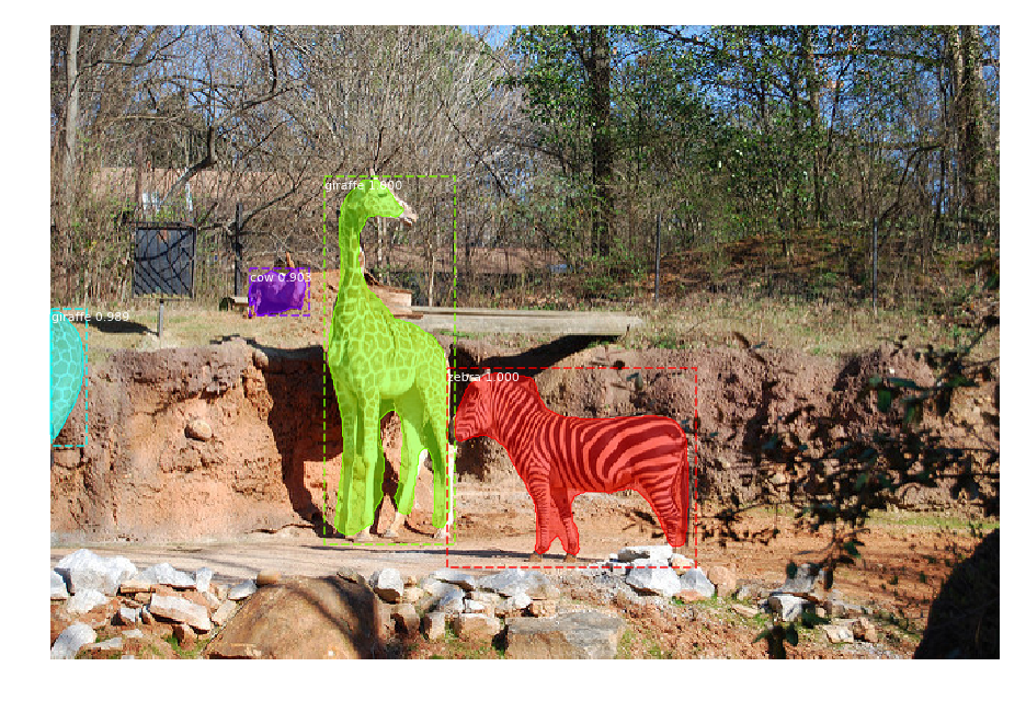 图:Mask RCNN检测效果
train_shapes.ipynb
除了可以使用训练好的模型,我们也可以用自己的数据进行训练,为了演示,这里使用了一个很小的shape数据集。这个数据集是on-the-fly的用代码生成的一些三角形、正方形、圆形,因此不需要下载数据。
配置
代码提供了基础的类Config,我们只需要继承并稍作修改:
class ShapesConfig(Config):
	"""用于训练shape数据集的配置
	继承子基本的Config类,然后override了一些配置项。
	"""
	# 起个好记的名字
	NAME = "shapes"

	# 使用一个GPU训练,每个GPU上8个图片。因此batch大小是8 (GPUs * images/GPU).
	GPU_COUNT = 1
	IMAGES_PER_GPU = 8

	# 分类数(需要包括背景类)
	NUM_CLASSES = 1 + 3  # background + 3 shapes

	# 图片为固定的128x128
	IMAGE_MIN_DIM = 128
	IMAGE_MAX_DIM = 128

	# 因为图片比较小,所以RPN anchor也是比较小的
	RPN_ANCHOR_SCALES = (8, 16, 32, 64, 128)  # anchor side in pixels

	# 每张图片建议的RoI数量,对于这个小图片的例子可以取比较小的值。
	TRAIN_ROIS_PER_IMAGE = 32

	# 每个epoch的数据量
	STEPS_PER_EPOCH = 100

	# 每5步验证一下。
	VALIDATION_STEPS = 5

config = ShapesConfig()
config.display()
Dataset
对于我们自己的数据集,我们需要继承utils.Dataset类,并且重写如下方法:
- load_image
- load_mask
- image_reference
在重写这3个方法之前我们首先来看load_shapes,这个函数on-the-fly的生成数据。
class ShapesDataset(utils.Dataset):
	"""随机生成shape数据。包括三角形,正方形和圆形,以及它的位置。
	这是on-th-fly的生成数据,因此不需要访问文件。
	"""

	def load_shapes(self, count, height, width):
		"""生成图片
		count: 返回的图片数量
		height, width: 生成图片的height和width
		"""
		# 类别
		self.add_class("shapes", 1, "square")
		self.add_class("shapes", 2, "circle")
		self.add_class("shapes", 3, "triangle")

		# 注意:这里只是生成图片的specifications(说明书),
		# 具体包括性质、颜色、大小和位置等信息。
		# 真正的图片是在load_image()函数里根据这些specifications
		# 来on-th-fly的生成。
		for i in range(count):
			bg_color, shapes = self.random_image(height, width)
			self.add_image("shapes", image_id=i, path=None,
				width=width, height=height,
				bg_color=bg_color, shapes=shapes)
其中add_image是在基类中定义:
def add_image(self, source, image_id, path, **kwargs):
    image_info = {
	    "id": image_id,
	    "source": source,
	    "path": path,
    }
    image_info.update(kwargs)
    self.image_info.append(image_info)
它有3个命名参数source、image_id和path。source是标识图片的来源,我们这里都是固定的字符串”shapes”;image_id是图片的id,我们这里用生成的序号i,而path一般标识图片的路径,我们这里是None。其余的参数就原封不动的保存下来。
random_image函数随机的生成图片的位置,请读者仔细阅读代码注释。
def random_image(self, height, width):
    """随机的生成一个specifications
    它包括图片的背景演示和一些(最多4个)不同的shape的specifications。
    """
    # 随机选择背景颜色
    bg_color = np.array([random.randint(0, 255) for _ in range(3)])
    # 随机生成一些(最多4个)shape
    shapes = []
    boxes = []
    N = random.randint(1, 4)
    for _ in range(N):
	    # random_shape函数随机产生一个shape(比如圆形),它的颜色和位置
	    shape, color, dims = self.random_shape(height, width)
	    shapes.append((shape, color, dims))
	    # 位置是中心点和大小(正方形,圆形和等边三角形只需要一个值表示大小)
	    x, y, s = dims
	    # 根据中心点和大小计算bounding box
	    boxes.append([y-s, x-s, y+s, x+s])
    # 使用non-max suppression去掉重叠很严重的图片
    keep_ixs = utils.non_max_suppression(np.array(boxes), np.arange(N), 0.3)
    shapes = [s for i, s in enumerate(shapes) if i in keep_ixs]
    return bg_color, shapes
随机生成一个shape的函数是random_shape:
def random_shape(self, height, width):
    """随机生成一个shape的specifications,
    要求这个shape在height和width的范围内。
    返回一个3-tuple:
    * shape名字 (square, circle, ...)
    * shape的颜色:代表RGB的3-tuple
    * shape的大小,一个数值
    """
    # 随机选择shape的名字
    shape = random.choice(["square", "circle", "triangle"])
    # 随机选择颜色
    color = tuple([random.randint(0, 255) for _ in range(3)])
    # 随机选择中心点位置,在范围[buffer, height/widht - buffer -1]内随机选择
    buffer = 20
    y = random.randint(buffer, height - buffer - 1)
    x = random.randint(buffer, width - buffer - 1)
    # 随机的大小size
    s = random.randint(buffer, height//4)
    return shape, color, (x, y, s)
上面的函数是我们为了生成(或者读取磁盘的图片)而写的代码。接下来我们需要重写上面的三个函数,我们首先来看load_image:
def load_image(self, image_id):
    """根据specs生成实际的图片
    如果是实际的数据集,通常是从一个文件读取。
    """
    info = self.image_info[image_id]
    bg_color = np.array(info['bg_color']).reshape([1, 1, 3])
    # 首先填充背景色
    image = np.ones([info['height'], info['width'], 3], dtype=np.uint8)
    image = image * bg_color.astype(np.uint8)
    # 分别绘制每一个shape
    for shape, color, dims in info['shapes']:
	    image = self.draw_shape(image, shape, dims, color)
    return image
上面的函数会调用draw_shape来绘制一个shape:
def draw_shape(self, image, shape, dims, color):
    """根据specs绘制shape"""
    # 获取中心点x, y和size s
    x, y, s = dims
    if shape == 'square':
	    cv2.rectangle(image, (x-s, y-s), (x+s, y+s), color, -1)
    elif shape == "circle":
	    cv2.circle(image, (x, y), s, color, -1)
    elif shape == "triangle":
	    points = np.array([[(x, y-s),
		    (x-s/math.sin(math.radians(60)), y+s),
		    (x+s/math.sin(math.radians(60)), y+s),
		    ]], dtype=np.int32)
	    cv2.fillPoly(image, points, color)
    return image
这个函数很直白,使用opencv的函数在image上绘图,正方形和圆形都很简单,就是等边三角形根据中心点和size(中心点到顶点的距离)求3个顶点的坐标需要一些平面几何的知识。
接下来是load_mask函数,这个函数需要返回图片中的目标物体的mask。这里需要稍作说明。通常的实例分隔数据集同时提供Bounding box和Mask(Bounding的某个像素是否属于目标物体)。为了更加通用,这里假设我们值提供Mask(也就是物体包含的像素),而Bounding box就是包含这些Mask的最小的长方形框,因此不需要提供。
对于我们随机生成的性质,只要知道哪种shape以及中心点和size,我们可以计算出这个物体(shape)到底包含哪些像素。对于真实的数据集,这通常是人工标注出来的。
def load_mask(self, image_id):
    """生成给定图片的mask
    """
    info = self.image_info[image_id]
    shapes = info['shapes']
    count = len(shapes)
    # 每个物体都有一个mask矩阵,大小是height x width
    mask = np.zeros([info['height'], info['width'], count], dtype=np.uint8)
    for i, (shape, _, dims) in enumerate(info['shapes']):
	    # 绘图函数draw_shape已经把mask绘制出来了。我们只需要传入特殊颜色值1。
	    mask[:, :, i:i+1] = self.draw_shape(mask[:, :, i:i+1].copy(),
		    shape, dims, 1)
    # 处理遮挡(occlusions)
    occlusion = np.logical_not(mask[:, :, -1]).astype(np.uint8)
    for i in range(count-2, -1, -1):
	    mask[:, :, i] = mask[:, :, i] * occlusion
	    occlusion = np.logical_and(occlusion, np.logical_not(mask[:, :, i]))
    # 类名到id
    class_ids = np.array([self.class_names.index(s[0]) for s in shapes])
    return mask.astype(np.bool), class_ids.astype(np.int32)
处理遮挡的代码可能有些tricky,不过这都不重要,因为通常的训练数据都是人工标注的,我们只需要从文件读取就行。这里我们值需要知道返回值的shape和含义就足够了。最后是image_reference函数,它的输入是image_id,输出是正确的分类。
def image_reference(self, image_id):
    info = self.image_info[image_id]
    if info["source"] == "shapes":
	    return info["shapes"]
    else:
	    super(self.__class__).image_reference(self, image_id)
上面的代码还判断了一些info[“source”],如果是”shapes”,说明是我们生成的图片,直接返回shape的名字,否则调用基类的image_reference。下面我们来生成一些图片看看。
# 训练集500个图片
dataset_train = ShapesDataset()
dataset_train.load_shapes(500, config.IMAGE_SHAPE[0], config.IMAGE_SHAPE[1])
dataset_train.prepare()

# 验证集50个图片
dataset_val = ShapesDataset()
dataset_val.load_shapes(50, config.IMAGE_SHAPE[0], config.IMAGE_SHAPE[1])
dataset_val.prepare()
image_ids = np.random.choice(dataset_train.image_ids, 4)
for image_id in image_ids:
	image = dataset_train.load_image(image_id)
	mask, class_ids = dataset_train.load_mask(image_id)
	visualize.display_top_masks(image, mask, class_ids, dataset_train.class_names)
随机生成的图片如下图所示,注意,因为每次都是随机生成,因此读者得到的结果可能是不同的。左图是生成的图片,右边是mask。
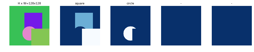 图:随机生成的Shape图片
创建模型
model = modellib.MaskRCNN(mode="training", config=config,
		model_dir=MODEL_DIR)
因为我们的训练数据不多,因此使用预训练的模型进行Transfer Learning会效果更好。
# 默认使用coco模型来初始化
init_with = "coco"  # imagenet, coco, or last

if init_with == "imagenet":
	model.load_weights(model.get_imagenet_weights(), by_name=True)
elif init_with == "coco":
	# 加载COCO模型的参数,去掉全连接层(mrcnn_bbox_fc),
	# logits(mrcnn_class_logits)
	# 输出的boudning box(mrcnn_bbox)和Mask(mrcnn_mask)
	model.load_weights(COCO_MODEL_PATH, by_name=True,
		exclude=["mrcnn_class_logits", "mrcnn_bbox_fc",
		"mrcnn_bbox", "mrcnn_mask"])
elif init_with == "last":
	# 加载我们最近训练的模型来初始化
	model.load_weights(model.find_last(), by_name=True)
训练
训练分为两个阶段:
- heads 只训练上面没有初始化的4层网络的参数,适合训练数据较少(比如本例子)的情况
- all 训练所有的参数
我们这里值训练heads就够了。
model.train(dataset_train, dataset_val,
		learning_rate=config.LEARNING_RATE,
		epochs=1,
		layers='heads')
保存模型参数:
# 手动保存参数,这通常是不需要的,
# 因为每次epoch介绍会自动保存,所以这里是注释掉的。
# model_path = os.path.join(MODEL_DIR, "mask_rcnn_shapes.h5")
# model.keras_model.save_weights(model_path)
检测
我们首先需要构造预测的Config并且加载模型参数。
class InferenceConfig(ShapesConfig):
	GPU_COUNT = 1
	IMAGES_PER_GPU = 1

inference_config = InferenceConfig()

# 重新构建用于inference的模型
model = modellib.MaskRCNN(mode="inference",
		config=inference_config,
		model_dir=MODEL_DIR)

# 加载模型参数,可以手动指定也可以让它自己找最近的模型参数文件
# model_path = os.path.join(ROOT_DIR, ".h5 file name here")
model_path = model.find_last()

# 加载模型参数
print("Loading weights from ", model_path)
model.load_weights(model_path, by_name=True)
我们随机寻找一个图片来检测:
# 随机选择验证集的一张图片。
image_id = random.choice(dataset_val.image_ids)
original_image, image_meta, gt_class_id, gt_bbox, gt_mask =\
	modellib.load_image_gt(dataset_val, inference_config,
		image_id, use_mini_mask=False)

log("original_image", original_image)
log("image_meta", image_meta)
log("gt_class_id", gt_class_id)
log("gt_bbox", gt_bbox)
log("gt_mask", gt_mask)

visualize.display_instances(original_image, gt_bbox, gt_mask, gt_class_id,
	dataset_train.class_names, figsize=(8, 8))
上面的代码加载一张图片,结果如下图所示,它显示的是真正的(gold/ground-truth) Bounding box和Mask。
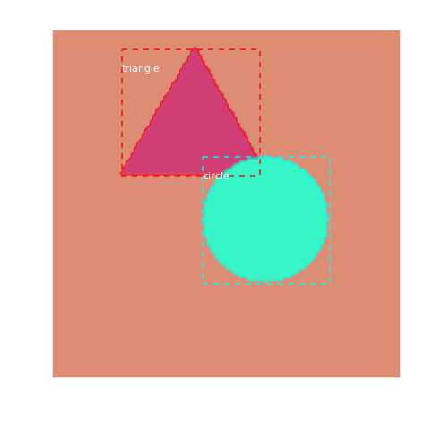 图:随机挑选的测试图片
接下来我们用模型来预测一下:
results = model.detect([original_image], verbose=1)

r = results[0]
visualize.display_instances(original_image, r['rois'], r['masks'], r['class_ids'],
	dataset_val.class_names, r['scores'], ax=get_ax())
模型预测的结果如下图所示,可以对比看成模型预测的非常准确。
 图:模型预测的结果
测试
前面我们只是测试了一个例子,我们需要更加全面的评测。
image_ids = np.random.choice(dataset_val.image_ids, 10)
APs = []
for image_id in image_ids:
	# 加载图片和正确的Bounding box以及mask
	image, image_meta, gt_class_id, gt_bbox, gt_mask =\
		modellib.load_image_gt(dataset_val, inference_config,
			image_id, use_mini_mask=False)
	molded_images = np.expand_dims(modellib.mold_image(image, inference_config), 0)
	# 进行检测
	results = model.detect([image], verbose=0)
	r = results[0]
	# 计算AP
	AP, precisions, recalls, overlaps =\
		utils.compute_ap(gt_bbox, gt_class_id, gt_mask,
			r["rois"], r["class_ids"], r["scores"], r['masks'])
	APs.append(AP)

print("mAP: ", np.mean(APs))
# 输出0.95
inspect_data.ipynb
这个notebook演示了Mask R-CNN的数据预处理过程。这个notebook可以用COCO数据集或者我们之前介绍的shape数据集进行演示,为了避免下载大量的COCO数据集,我们这里用shape数据集。
选择数据集
config = ShapesConfig()

# 我们把下面的代码注释掉
# MS COCO Dataset
#import coco
#config = coco.CocoConfig()
#COCO_DIR = "path to COCO dataset"  # TODO: enter value here
加载Dataset
# Load dataset
if config.NAME == 'shapes':
	dataset = ShapesDataset()
	dataset.load_shapes(500, config.IMAGE_SHAPE[0], config.IMAGE_SHAPE[1])
elif config.NAME == "coco":
	dataset = coco.CocoDataset()
	dataset.load_coco(COCO_DIR, "train")

# 使用dataset之前必须调用prepare()
dataset.prepare()

print("Image Count: {}".format(len(dataset.image_ids)))
print("Class Count: {}".format(dataset.num_classes))
for i, info in enumerate(dataset.class_info):
	print("{:3}. {:50}".format(i, info['name']))

# 运行后的结果为:
Image Count: 500
Class Count: 4
0. BG
1. square
2. circle
3. triangle
显示样本
我们可以显示一些样本。
image_ids = np.random.choice(dataset.image_ids, 4)
for image_id in image_ids:
	image = dataset.load_image(image_id)
	mask, class_ids = dataset.load_mask(image_id)
	visualize.display_top_masks(image, mask, class_ids, dataset.class_names)
结果如下图所示。
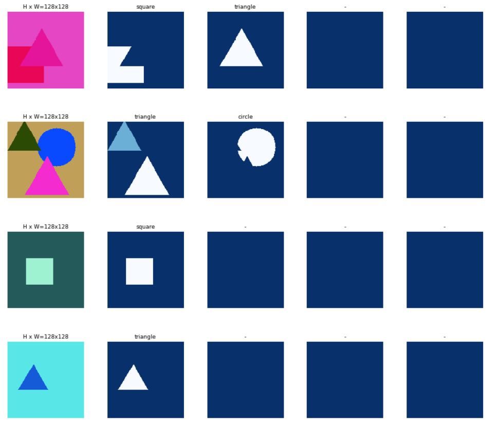 图:Mask 显示4个样本
Bounding Box
一般的数据集同时提供Bounding box和Mask,但是为了简单,我们只需要数据集提供Mask,我们可以通过Mask计算出Bounding box来。这样还有一个好处,那就是如果我们对目标物体进行旋转缩放等操作,计算Mask会比较容易,我们可以用新的Mask重新计算新的Bounding Box。否则我们就得对Bounding box进行相应的旋转缩放,这通常比较麻烦。
# 随机加载一个图片和它对应的mask.
image_id = random.choice(dataset.image_ids)
image = dataset.load_image(image_id)
mask, class_ids = dataset.load_mask(image_id)
# 计算Bounding box
bbox = utils.extract_bboxes(mask)

# 显示图片其它的统计信息
print("image_id ", image_id, dataset.image_reference(image_id))
log("image", image)
log("mask", mask)
log("class_ids", class_ids)
log("bbox", bbox)
# 显示图片
visualize.display_instances(image, bbox, mask, class_ids, dataset.class_names)
最重要的代码就是bbox = utils.extract_bboxes(mask)。最终得到的图片如下图所示。
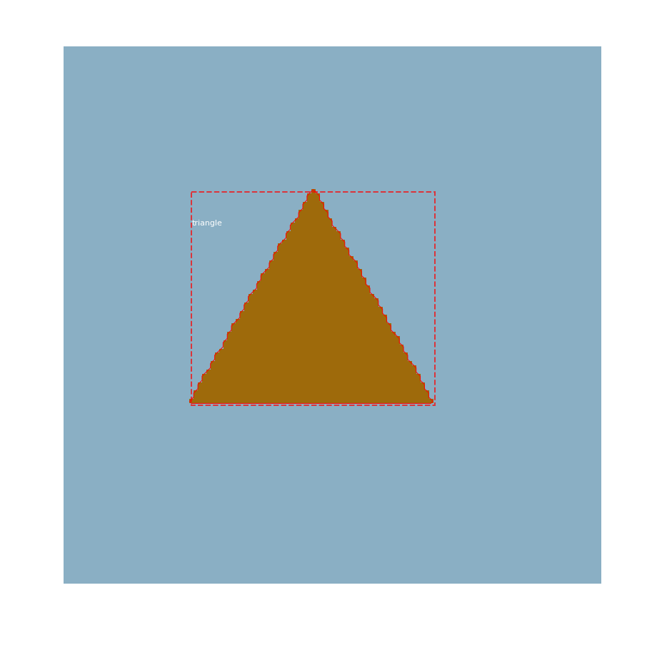 图:显示样本
\subsubsection{缩放图片} 我们需要把图片都缩放成1024x1024(shape数据是生成的,都是固定大小,但实际数据集肯定不是这样)。我们会保持宽高比比最大的缩放成1024,比如原来是512x256,那么就会缩放成1024x512。然后我们把不足的维度两边补零,比如把1024x512padding成1024x1024,height维度上下各补256个0(256个0+512个真实数据+256个0)。
# 随机加载一个图片和它的mask
image_id = np.random.choice(dataset.image_ids, 1)[0]
image = dataset.load_image(image_id)
mask, class_ids = dataset.load_mask(image_id)
original_shape = image.shape
# 缩放图片,
image, window, scale, padding, _ = utils.resize_image(
	image,
	min_dim=config.IMAGE_MIN_DIM,
	max_dim=config.IMAGE_MAX_DIM,
	mode=config.IMAGE_RESIZE_MODE)

# 缩放图片后一定要缩放mask,否则就不一致了
mask = utils.resize_mask(mask, scale, padding)
# 计算Bounding box
bbox = utils.extract_bboxes(mask)

# 显示图片的其它统计信息
print("image_id: ", image_id, dataset.image_reference(image_id))
print("Original shape: ", original_shape)
log("image", image)
log("mask", mask)
log("class_ids", class_ids)
log("bbox", bbox)

# 显示图片
visualize.display_instances(image, bbox, mask, class_ids, dataset.class_names)
Mini Masks
一个图片可能有多个目标物体,每个物体的Mask是一个bool数组,大小是[width, height]。很显然,Bounding box之外的Mask肯定都是False,如果物体的比较小的话,这么存储是比较浪费空间的。因此我们有如下改进方法:
- 我们只存储Bounding Box里的坐标对应的Mask值
- 我们把Mask缩小(比如56x56),用的时候在放大回去,这对大的目标物体会有误差。但是由于我们的(人工)标注本来就没那么准。
为了可视化Mask缩放,我们来看几个例子。
image_id = np.random.choice(dataset.image_ids, 1)[0]
image, image_meta, class_ids, bbox, mask = modellib.load_image_gt(
	dataset, config, image_id, use_mini_mask=False)

log("image", image)
log("image_meta", image_meta)
log("class_ids", class_ids)
log("bbox", bbox)
log("mask", mask)

display_images([image]+[mask[:,:,i] for i in range(min(mask.shape[-1], 7))])

# 输出
image                    shape: (128, 128, 3)         min:    4.00000  max:  241.00000  uint8
image_meta               shape: (16,)                 min:    0.00000  max:  409.00000  int64
class_ids                shape: (2,)                  min:    1.00000  max:    3.00000  int32
bbox                     shape: (2, 4)                min:   14.00000  max:  128.00000  int32
mask                     shape: (128, 128, 2)         min:    0.00000  max:    1.00000  bool
如下图所示,这个图片有一个正方形和一个三角形。
 图:显示样本
接下来我们对图片进行增强,比如镜像。
image, image_meta, class_ids, bbox, mask = modellib.load_image_gt(
	dataset, config, image_id, augment=True, use_mini_mask=True)
log("mask", mask)
display_images([image]+[mask[:,:,i] for i in range(min(mask.shape[-1], 7))])
上面调用函数modellib.load_image_gt,参数use_mini_mask设置为True。效果如下图所示。首先做了镜像对称变化,另外我们可以看到mask的shape从(128, 128, 2)变成了(56, 56, 2),而且mask都是Bounding Box里的mask。
 图:mini mask和增强
Anchor
anchor的顺序非常重要,训练和预测要使用相同的anchor序列。另外也要匹配卷积的运算顺序。对于一个FPN,anchor的顺序要便于卷积层的输出预测anchor的得分和位移(shift)。因此通常使用如下顺序:
- 首先安装金字塔的层级排序,首先是第一层,然后是第二层
- 对于同一层,安装卷积的顺序从左上到右下逐行排序
- 对于同一个点,按照宽高比(aspect ratio)排序
Anchor Stride:在FPN网络结构下,前几层的feature map是高分辨率的。比如输入图片是1024x1024,则第一层的feature map是256x256,这将产生大约200k个anchor(2562563),这些anchor是32x32的,而它们的stride是4个像素,因此会有大量重叠的anchor。如果我们每隔一个cell(而不是每个cell)生成一次anchor,这将极大降低计算量。这里使用的stride是2,这和论文使用的1不同。生成anchor的代码如下:
# Generate Anchors
backbone_shapes = modellib.compute_backbone_shapes(config, config.IMAGE_SHAPE)
anchors = utils.generate_pyramid_anchors(config.RPN_ANCHOR_SCALES,
	config.RPN_ANCHOR_RATIOS,
	backbone_shapes,
	config.BACKBONE_STRIDES,
	config.RPN_ANCHOR_STRIDE)

# 输出anchor的摘要信息
num_levels = len(backbone_shapes)
anchors_per_cell = len(config.RPN_ANCHOR_RATIOS)
print("Count: ", anchors.shape[0])
print("Scales: ", config.RPN_ANCHOR_SCALES)
print("ratios: ", config.RPN_ANCHOR_RATIOS)
print("Anchors per Cell: ", anchors_per_cell)
print("Levels: ", num_levels)
anchors_per_level = []
for l in range(num_levels):
	num_cells = backbone_shapes[l][0] * backbone_shapes[l][1]
	anchors_per_level.append(anchors_per_cell * num_cells //
		config.RPN_ANCHOR_STRIDE**2)
	print("Anchors in Level {}: {}".format(l, anchors_per_level[l]))
输出的统计信息是:
Count:  4092
Scales:  (8, 16, 32, 64, 128)
ratios:  [0.5, 1, 2]
Anchors per Cell:  3
Levels:  5
Anchors in Level 0: 3072
Anchors in Level 1: 768
Anchors in Level 2: 192
Anchors in Level 3: 48
Anchors in Level 4: 12
我们来分析一下,总共有5种scales。对于第0层,Feature map是32x32,每个cell有3种宽高比,因此总共有3072个anchor;而第一层的Feature map是16x16,所以有768个anchor。我们来看每一层的feature map中心cell的anchor。
## Visualize anchors of one cell at the center of the feature map of a specific level

# Load and draw random image
image_id = np.random.choice(dataset.image_ids, 1)[0]
image, image_meta, _, _, _ = modellib.load_image_gt(dataset, config, image_id)
fig, ax = plt.subplots(1, figsize=(10, 10))
ax.imshow(image)
levels = len(backbone_shapes)

for level in range(levels):
	colors = visualize.random_colors(levels)
	# Compute the index of the anchors at the center of the image
	level_start = sum(anchors_per_level[:level]) # sum of anchors of previous levels
	level_anchors = anchors[level_start:level_start+anchors_per_level[level]]
	print("Level {}. Anchors: {:6}  Feature map Shape: {}".format(level,
		level_anchors.shape[0], backbone_shapes[level]))
	center_cell = backbone_shapes[level] // 2
	center_cell_index = (center_cell[0] * backbone_shapes[level][1] + center_cell[1])
	level_center = center_cell_index * anchors_per_cell
	center_anchor = anchors_per_cell * (
		(center_cell[0] * backbone_shapes[level][1] / config.RPN_ANCHOR_STRIDE**2) \
		+ center_cell[1] / config.RPN_ANCHOR_STRIDE)
	level_center = int(center_anchor)

	# Draw anchors. Brightness show the order in the array, dark to bright.
	for i, rect in enumerate(level_anchors[level_center:level_center+anchors_per_cell]):
		y1, x1, y2, x2 = rect
		p = patches.Rectangle((x1, y1), x2-x1, y2-y1, linewidth=2, facecolor='none',
		edgecolor=(i+1)*np.array(colors[level]) / anchors_per_cell)
		ax.add_patch(p)
结果如下图所示。
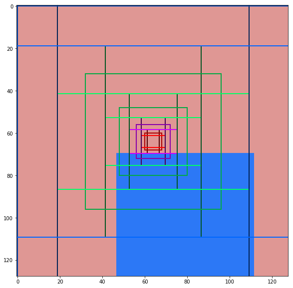 图:Anchor
训练数据生成器
我们在训练Mask R-CNN的时候,会计算候选的区域和真实的目标区域的IoU,从而选择正例和负例。
random_rois = 2000
g = modellib.data_generator(
	dataset, config, shuffle=True, random_rois=random_rois,
	batch_size=4,
	detection_targets=True)

# Get Next Image
if random_rois:
	[normalized_images, image_meta, rpn_match, rpn_bbox, gt_class_ids,
		gt_boxes, gt_masks, rpn_rois, rois],
	[mrcnn_class_ids, mrcnn_bbox, mrcnn_mask] = next(g)

	log("rois", rois)
	log("mrcnn_class_ids", mrcnn_class_ids)
	log("mrcnn_bbox", mrcnn_bbox)
	log("mrcnn_mask", mrcnn_mask)
else:
	[normalized_images, image_meta, rpn_match, rpn_bbox, gt_boxes, gt_masks], _ =
		next(g)

log("gt_class_ids", gt_class_ids)
log("gt_boxes", gt_boxes)
log("gt_masks", gt_masks)
log("rpn_match", rpn_match, )
log("rpn_bbox", rpn_bbox)
image_id = modellib.parse_image_meta(image_meta)["image_id"][0]
print("image_id: ", image_id, dataset.image_reference(image_id))

# Remove the last dim in mrcnn_class_ids. It's only added
# to satisfy Keras restriction on target shape.
mrcnn_class_ids = mrcnn_class_ids[:,:,0]

b = 0

# Restore original image (reverse normalization)
sample_image = modellib.unmold_image(normalized_images[b], config)

# Compute anchor shifts.
indices = np.where(rpn_match[b] == 1)[0]
refined_anchors = utils.apply_box_deltas(anchors[indices], rpn_bbox[b, :len(indices)]
			* config.RPN_BBOX_STD_DEV)
log("anchors", anchors)
log("refined_anchors", refined_anchors)

# Get list of positive anchors
positive_anchor_ids = np.where(rpn_match[b] == 1)[0]
print("Positive anchors: {}".format(len(positive_anchor_ids)))
negative_anchor_ids = np.where(rpn_match[b] == -1)[0]
print("Negative anchors: {}".format(len(negative_anchor_ids)))
neutral_anchor_ids = np.where(rpn_match[b] == 0)[0]
print("Neutral anchors: {}".format(len(neutral_anchor_ids)))

# ROI breakdown by class
for c, n in zip(dataset.class_names, np.bincount(mrcnn_class_ids[b].flatten())):
	if n:
		print("{:23}: {}".format(c[:20], n))

# Show positive anchors
visualize.draw_boxes(sample_image, boxes=anchors[positive_anchor_ids],
refined_boxes=refined_anchors)
输出为:
anchors                  shape: (4092, 4)             min:  -90.50967  max:  154.50967  float64
refined_anchors          shape: (3, 4)                min:    6.00000  max:  128.00000  float32
Positive anchors: 3
Negative anchors: 253
Neutral anchors: 3836
BG                     : 22
square                 : 1
circle                 : 9
对于随机的一个图片,这里生成了4092个anchor,其中3个正样本,253个负样本,其余的都是无用的样本。下图是3个正样本;下图是负样本;而下图是无用的数据。
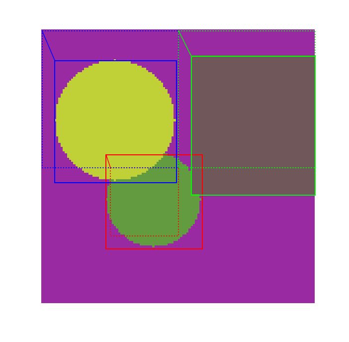 图:正样本anchor
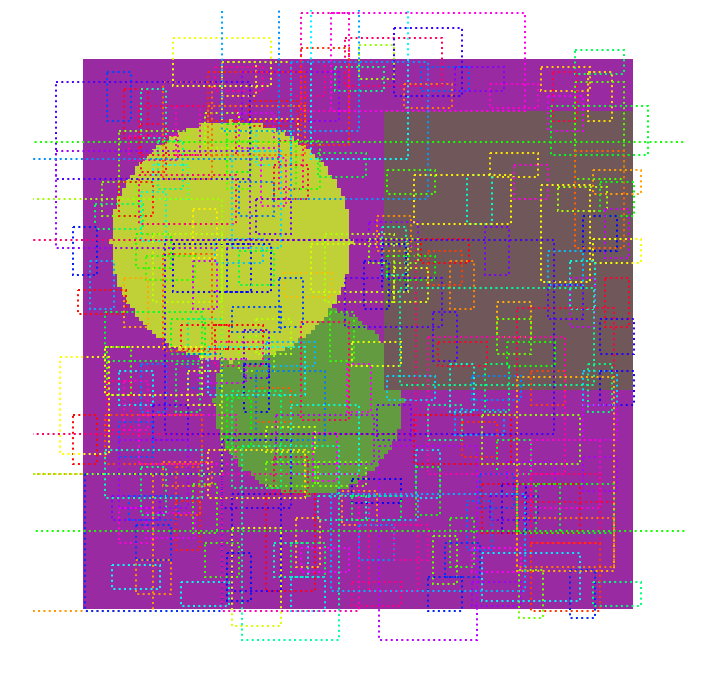 图:负样本anchor
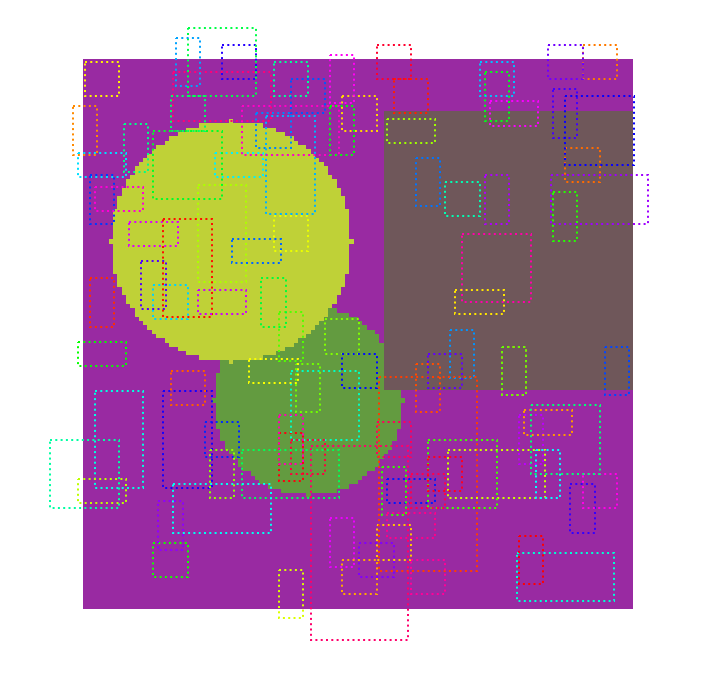 图:无用的anchor
- 显示Disqus评论(需要科学上网)