本文介绍XLNet的代码的第三部分,需要首先阅读第一部分和第二部分,读者阅读前需要了解XLNet的原理,不熟悉的读者请先阅读XLNet原理。
目录
transformer_xl构造函数
第五段
    ##### 位置编码,下面我们会详细介绍,它的输出是(352, 8, 1024)
    pos_emb = relative_positional_encoding(
        qlen, klen, d_model, clamp_len, attn_type, bi_data,
        bsz=bsz, dtype=tf_float)
    # dropout
    pos_emb = tf.layers.dropout(pos_emb, dropout, training=is_training)
相对位置编码的基本概念
这里是相对位置编码,注意这里的”相对”位置指的是两个位置的差,而不是Transformer里的相对位置编码。
BERT是使用”绝对”位置编码,它把每一个位置都编码成一个向量。而在Transformer里,每个位置还是编码成一个向量,不过这个向量是固定的,而且是正弦(余弦)的函数形式,这样上层可以通过它来学习两个词的相对位置的关系,具体读者可以参考Transformer代码阅读。
而这里的”相对”位置编码是Transformer-XL里提出的一种更加一般的位置编码方式(作者在XLNet原理里的说法是不正确的,当时只是阅读了论文,没有详细看代码)。
而Transformer-XL(包括follow它的XLNet)为什么又要使用一种新的”相对”位置编码呢?这是由于Transformer-XL引入了之前的context(cache)带来的问题。
在标准的Transformer里,如果使用绝对位置编码,假设最大的序列长度为$L_{max}$,则只需要一个位置编码矩阵$U \in R^{L_{max}\times d}$,其中$U_i$表示第i个位置的Embedding。而Transformer的第一层的输入是Word Embedding加上Position Embedding,从而把位置信息输入给了Transformer,这样它的Attention Head能利用这里面包含的位置信息。那Transformer-XL如果直接使用这种编码方式行不行呢?我们来试一下:
和前面一样,假设两个相邻的segment为$s_\tau=[x_{\tau,1}, x_{\tau,2}, …, x_{\tau,L}]$和$s_{\tau+1}=[x_{\tau+1,1}, x_{\tau+1,2}, …, x_{\tau+1,L}]$。假设segment $s_\tau$的第n层的隐状态序列为$h_\tau^n \in R^{L \times d}$,那么计算公式如下:
\[\begin{split} h_{\tau+1} & =f(h_\tau,E_{s_{\tau+1}} + U_{1:L}) \\ h_{\tau} & =f(h_{\tau-1},E_{s_{\tau}} + U_{1:L}) \end{split}\]上式中$E_{s_{\tau}}$是segment的每一个词的Embedding的序列。我们发现$E_{s_{\tau}}$和$E_{s_{\tau+1}}$都是加了$U_{1:L}$,因此假设模型发现了输入有这个向量(包含),那么它也无法通过这个向量判断到底是当前segment的第i个位置还是前一个segment的第i个位置。
举个例子:比如一种情况是”a b c | d e f”(它表示context是”a b c”,当前输入是”d e f”);第二种情况是”d b c | a e f”。那么在第二个时刻,这两种情况计算e到a的attention时都是用e的Embedding(Word Embedding+Position Embedding)去乘以a的Embedding(WordEmbedding+Position Embedding)【当然实际还要把它们经过Q和K变换矩阵,但是这不影响结论】,因此计算结果是相同的,但是实际上一个a是在它的前面,而另一个a是在很远的context里。
因此我们发现问题的关键是Transformer使用的是一种”绝对”位置的编码(之前的那种使用正弦函数依然是绝对位置编码,但是它能够让上层学习到两个位置的相对信息,所以当时也叫作相对位置编码。但是对于一个位置,它还是一个固定的编码,请一定要搞清楚)。
为了解决这个问题,Transformer-XL引入了”真正”的相对位置编码方法。它不是把位置信息提前编码在输入的Embedding里,而是在计算attention的时候根据当前的位置和要attend to的位置的相对距离来”实时”告诉attention head。比如当前的query是$q_{\tau,i}$,要attend to的key是$k_{\tau,j}$,那么只需要知道i和j的位置差,然后就可以使用这个位置差的位置Embedding。
我们回到前面的例子,context大小是96,而输入的序列长度是128。因此query的下标i的取值范围是96-223,而key的下标j的取值范围是0-223,所以它们的差的取值范围是(96-223)-(223-0),所以位置差总共有352种可能的取值,所以上面返回的pos_emb的shape是(352, 8, 1024)。
下面是详细的相对位置编码的原理和代码,不感兴趣的读者可以跳过,但是至少需要知道前面的基本概念以及pos_emb的shape的含义。
相对位置编码的详细计算过程
在标准的Transformer里,同一个segment的$q_i$和$k_j$的attention score可以这样分解:
\[\begin{split} A_{i,j}^{abs} & = \underbrace{E^T_{x_i}W_q^TW_kE_{x_j}}_{(a)}+\underbrace{E^T_{x_i}W_q^TW_kU_j}_{(b)} \\ & + \underbrace{U_i^TW_q^TW_kE_{x_j}}_{(c)}+\underbrace{U_i^TW_q^TW_kU_j}_{(d)} \end{split}\]参考上面的公式,并且因为希望只考虑相对的位置,所以我们(Transformer-XL)提出如下的相对位置Attention计算公式:
\[\begin{split} A_{i,j}^{rel} & = \underbrace{E^T_{x_i}W_q^TW_{k,E}E_{x_j}}_{(a)}+\underbrace{E^T_{x_i}W_q^TW_{k,R}\color{blue}{R_{i-j}}}_{(b)} \\ & + \underbrace{\color{red}{u^T}W_{k,E}E_{x_j}}_{(c)} + \underbrace{\color{red}{v^T}W_{k,R}\color{blue}{R_{i-j}}}_{(d)} \end{split}\]-
和前面的$A_{i,j}^{abs}$相比,第一个是把(b)和(d)里的绝对位置编码$U_j$都替换成相对位置编码向量$R_{i-j}$。注意这里的R是之前介绍的”相对”的正弦函数的编码方式,它是固定的没有可以学习的参数。
-
在(c)中用可训练的$\color{red}{u} \in R^d$替代原来的$U_i^TW_q^T$。因为我们假设Attention score只依赖于i和j的相对位置,而与i的绝对位置无关,所以这里对于所有i都相同。也就是$U^TW_q^T$,所以可以用一个新的$\color{red}{u}$来表示。类似的是(d)中的$\color{red}{v} \in R^d$。
-
最后,我们把key的变换矩阵$W_k$拆分成$W_{k,E}$和$W_{k,R}$,分别表示与内容相关的key和与位置相关的key。
在上面的新公式里,每一项的意义都非常清晰:(a)表示内容的计算,也就是$x_i$的Embedding乘以变换矩阵$W_q$和$x_j$的Embedding乘以$W_{k,E}$的内积;(b)表示基于内容的位置偏置,也就是i的向量乘以相对位置编码;(c)全局的内容偏置;(d)全局的位置偏置。
因此Transformer-XL里的计算过程如下:
\[\begin{split} \hat{h}_{\tau}^{n-1} & = [SG(m_{\tau}^{n-1} \circ h_{\tau}^{n-1})] \\ q_{\tau}^n, k_{\tau}^n, v_{\tau}^n & = h_{\tau}^{n-1}{W_q^n}^T, \hat{h}_{\tau}^{n-1} {W_{k,E}^n}^T, \hat{h}_{\tau}^{n-1} {W_{v}^n}^T \\ A_{\tau, i,j}^n & = {q_{\tau,i}^n}^T k_{\tau,j}^n + {q_{\tau,i}^n}^T W_{k,R}^nR_{i-j} \\ & + u^Tk_{\tau,j}^n +v^T W_{k,R}^nR_{i-j} \\ a_\tau^n & = \text{Mask-Softmax}(A_\tau^n)v_\tau^n \\ o_\tau^n & = \text{LayerNorm}(\text{Linear}(a_\tau^n)+h_\tau^{n-1}) \\ h_\tau^n & = \text{Positionwise-Feed-Forward}(o_\tau^n) \end{split}\]- 第一个等式说明当前的输入是memory($m_{\tau}^{n-1}$)和上一个时刻的隐状态$h_{\tau}^{n-1}$,SG()的意思是不参与梯度计算。$\circ$表示向量拼接。
- 第二个等式计算query、key和value,其中query只能用上一个时刻的隐状态$h_{\tau}^{n-1}$,而key和value是使用上面的\(\hat{h}_{\tau}^{n-1}\)。因为Key分成了$W_{k,E}$和$W_{k,R}$,这里只用表示内容的$W_{k,E}$。
- 第三个公式根据前面的$A^{rel}$计算attention得分。基本和上式相同,只不过$EW$都已经计算到q,k和v里了,所以用它们替代就行。
- 第四个公式用softmax把score变成概率,需要处理Mask(mask的概率为0)
- 第五个公式是残差连接和LayerNorm
- 最后是全连接层
接下来我们看怎么获得相对位置编码,注意,上面的计算过程要在后面才会介绍。
relative_positional_encoding函数
def relative_positional_encoding(qlen, klen, d_model, clamp_len, attn_type,
                                 bi_data, bsz=None, dtype=None):
  """创建相对位置编码"""
  # [0,2,...,1022] 长度为d_model/2=512
  freq_seq = tf.range(0, d_model, 2.0)
  if dtype is not None and dtype != tf.float32:
    freq_seq = tf.cast(freq_seq, dtype=dtype)
  # inv_freq的大小还是512
  inv_freq = 1 / (10000 ** (freq_seq / d_model))

  if attn_type == 'bi':
    # 我们这里attn_type == 'bi'
    # beg, end = 224, -128
    beg, end = klen, -qlen
  elif attn_type == 'uni':
    # beg, end = klen - 1, -1
    beg, end = klen, -1
  else:
    raise ValueError('Unknown `attn_type` {}.'.format(attn_type))

  if bi_data:
    # [224, -127]
    fwd_pos_seq = tf.range(beg, end, -1.0)
    # [-224, 127]
    bwd_pos_seq = tf.range(-beg, -end, 1.0)

    if dtype is not None and dtype != tf.float32:
      fwd_pos_seq = tf.cast(fwd_pos_seq, dtype=dtype)
      bwd_pos_seq = tf.cast(bwd_pos_seq, dtype=dtype)

    if clamp_len > 0:
      # 把两个词的最大距离限制在-clamp_len和clamp_len之间,我们这里没有限制
      fwd_pos_seq = tf.clip_by_value(fwd_pos_seq, -clamp_len, clamp_len)
      bwd_pos_seq = tf.clip_by_value(bwd_pos_seq, -clamp_len, clamp_len)

    if bsz is not None:
      # 参考下面,它的返回是(352, 4, 1024)
      fwd_pos_emb = positional_embedding(fwd_pos_seq, inv_freq, bsz//2)
      # 返回(352, 4, 1024)
      bwd_pos_emb = positional_embedding(bwd_pos_seq, inv_freq, bsz//2)
    else:
      fwd_pos_emb = positional_embedding(fwd_pos_seq, inv_freq)
      bwd_pos_emb = positional_embedding(bwd_pos_seq, inv_freq)
    # (352, 8, 1024)
    pos_emb = tf.concat([fwd_pos_emb, bwd_pos_emb], axis=1)
  else:
    fwd_pos_seq = tf.range(beg, end, -1.0)
    if dtype is not None and dtype != tf.float32:
      fwd_pos_seq = tf.cast(fwd_pos_seq, dtype=dtype)
    if clamp_len > 0:
      fwd_pos_seq = tf.clip_by_value(fwd_pos_seq, -clamp_len, clamp_len)
    pos_emb = positional_embedding(fwd_pos_seq, inv_freq, bsz)

  return pos_emb
这个函数返回相对位置的编码,它返回一个(352, 8, 1024)的Tensor。8表示batch,1024表示位置编码的维度,它是和隐单元相同大小,这样可以相加(残差连接)。
前面我们介绍过,这里再复述一下。context大小是96,而输入的序列长度是128。因此query的下标i的取值范围是96-223,而key的下标j的取值范围是0-223,所以它们的差的取值范围是(96-223)-(223-0),所以位置差总共有352种可能的取值,所以上面返回的pos_emb的shape是(352, 8, 1024)。fwd_pos_seq的范围是[224, -127],表示当i>=j时(从后往前)从i attend to j的最大范围是223 attend to 0(加上attend to 自己总共224个可能取值);而i<j时最小值是-127。参考下图:
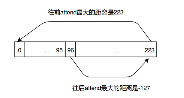 图:相对位置编码的attend范围
计算正弦的位置编码是通过下面介绍的函数positional_embedding来实现的,读者可以对照Transformer代码阅读·位置编码来阅读,那里是PyTorch的实现。
tf.einsum函数
在介绍positional_embedding函数之前我们介绍一下Tensorflow的einsum函数,这个函数在下面很多地方都会用到,所以这里单独作为一个小节来介绍一下。
这个函数返回一个Tensor,这个Tensor的元素由Einstein summation习惯的简写公式定义。所谓的Einstein summation指的是由Albert Einstein引入的一种公式简写法。比如计算矩阵A和B的乘积得到C。则C的元素的定义为:
C[i,k] = sum_j A[i,j] * B[j,k]
如果读者熟悉Latex的公式,则上面内容在Latex里会显示为:
\[C[i,k] = \sum_j A[i,j] * B[j,k]\]上面的这个公式简写为:
ij,jk->ik
那这种简写方法是什么意思呢?或者说怎么从上面的公式得到简写的呢?它的过程如下:
- 删除变量、括号和逗号
- 把”*“变成”,”
- 去掉求和符号
- 把输出移动右边,把”=”变成”->”
下面我们按照前面的4个步骤看看这个过程:
C[i,k] = sum_j A[i,j] * B[j,k] 删除变量、括号和逗号变成,
ik = sum_j ij * jk 把"*"变成","
ik = sum_j ij , jk 去掉求和符号
ik = ij,jk 把输出放到右边,把"="变成"->"
ij,jk->ik
下面我们来看一些例子,请读者理解它们的含义,如果不理解,可以按照前面的方法一步一步来。
# 矩阵乘法,这个前面已经介绍过
>>> einsum('ij,jk->ik', m0, m1)  # output[i,k] = sum_j m0[i,j] * m1[j, k]

# 向量的内积,注意输出是空,表示输出没有下标,因为输出是一个数值。
>>> einsum('i,i->', u, v)  # output = sum_i u[i]*v[i]

# 向量外积
>>> einsum('i,j->ij', u, v)  # output[i,j] = u[i]*v[j]

# 矩阵转置
>>> einsum('ij->ji', m)  # output[j,i] = m[i,j]

# Batch 矩阵乘法
>>> einsum('aij,ajk->aik', s, t)  # out[a,i,k] = sum_j s[a,i,j] * t[a, j, k]
positional_embedding
def positional_embedding(pos_seq, inv_freq, bsz=None):
  # 计算pos_seq和inv_freq的外积
  # 352 x 512
  sinusoid_inp = tf.einsum('i,d->id', pos_seq, inv_freq)
  # 计算sin和cos,然后拼接成(352, 1024)
  pos_emb = tf.concat([tf.sin(sinusoid_inp), tf.cos(sinusoid_inp)], -1)
  # 变成(352, 1, 1024) 如果不懂None的含义请参考第二部分
  # 它等价于tf.reshape(pos_emb, [352, 1, 1024])
  pos_emb = pos_emb[:, None, :]

  if bsz is not None:
    # 对每个batch复制,变成(352, 8, 1024)
    pos_emb = tf.tile(pos_emb, [1, bsz, 1])

  return pos_emb
相对位置编码向量的获得就介绍到这,后面在Attention的计算是会用到pos_emb,我们到时候再看具体的计算。
第六段
这一对是核心的计算two stream attention的地方。
    ##### Attention layers
    if mems is None:
      mems = [None] * n_layer

    for i in range(n_layer):
      # 通过当前的输出计算新的mem,也就是保留128个中的后96个
      # 当然如果cache的大小大于当前的输入,那么mem里可能包含当前输入的全部以及之前的mem
      new_mems.append(_cache_mem(output_h, mems[i], mem_len, reuse_len))

      # segment bias
      if seg_id is None:
        r_s_bias_i = None
        seg_embed_i = None
      else:
        # 这里是不共享bias的,所以从r_s_bias(6, 16, 64)取出
        # 当前层的bias(16, 64)
        r_s_bias_i = r_s_bias if not untie_r else r_s_bias[i]
        # 从(6, 2, 16, 64)取出当前层的segment embedding
        # seg_embed_i为(2, 16, 64)
        seg_embed_i = seg_embed[i]

      with tf.variable_scope('layer_{}'.format(i)):
        # inp_q表示哪些位置是Mask从而计算loss,也表示这是Pretraining
        if inp_q is not None:
          # 这是计算two stream attention,下面会详细介绍
          # 它的返回值output_h表示
          # output_g表示
          output_h, output_g = two_stream_rel_attn(
              h=output_h,
              g=output_g,
              r=pos_emb,
              r_w_bias=r_w_bias if not untie_r else r_w_bias[i],
              r_r_bias=r_r_bias if not untie_r else r_r_bias[i],
              seg_mat=seg_mat,
              r_s_bias=r_s_bias_i,
              seg_embed=seg_embed_i,
              attn_mask_h=non_tgt_mask,
              attn_mask_g=attn_mask,
              mems=mems[i],
              target_mapping=target_mapping,
              d_model=d_model,
              n_head=n_head,
              d_head=d_head,
              dropout=dropout,
              dropatt=dropatt,
              is_training=is_training,
              kernel_initializer=initializer)
          reuse = True
        else:
          reuse = False

          output_h = rel_multihead_attn(
              h=output_h,
              r=pos_emb,
              r_w_bias=r_w_bias if not untie_r else r_w_bias[i],
              r_r_bias=r_r_bias if not untie_r else r_r_bias[i],
              seg_mat=seg_mat,
              r_s_bias=r_s_bias_i,
              seg_embed=seg_embed_i,
              attn_mask=non_tgt_mask,
              mems=mems[i],
              d_model=d_model,
              n_head=n_head,
              d_head=d_head,
              dropout=dropout,
              dropatt=dropatt,
              is_training=is_training,
              kernel_initializer=initializer,
              reuse=reuse)
这段代码把下一层的输出更新mem,然后把它作为上一层的输入。核心是使用two_stream_rel_attn函数计算Attention。我们先看mem的更新。
_cache_mem函数
_cache_mem函数代码如下:
def _cache_mem(curr_out, prev_mem, mem_len, reuse_len=None):
  """把隐状态chache进memory"""
  if mem_len is None or mem_len == 0:
    return None
  else:
    if reuse_len is not None and reuse_len > 0:
      # reuse的部分cache,curr_out从(128,...)变成(64,....)
      # 原因是生成数据时我们每次后移64,请参考第一部分代码
      curr_out = curr_out[:reuse_len]

    if prev_mem is None:
      new_mem = curr_out[-mem_len:]
    else:
      #之前的mem(96)和当前的输出(64)拼起来然后取后面mem_len(96)个
      new_mem = tf.concat([prev_mem, curr_out], 0)[-mem_len:]

  # cache的mem不参与梯度计算
  return tf.stop_gradient(new_mem)
two_stream_rel_attn函数
我们先看输入参数:
- h (128, 8, 1024) 上一层的内容(context)隐状态
- g (21, 8, 1204) 上一层的查询(query)隐状态,只需要计算Mask的哪些位置
- r (352, 8, 1024) 相对位置编码,函数relative_positional_encoding的返回值
- r_w_bias (16, 64)
- r_r_bias (16, 64)
- seg_mat (128, 224, 8, 2) 表示i(范围是0-127)和j(被attend to的,包括mem因此范围是0-223)是否在同一个segment里,1是True
- r_s_bias (16, 64)
- seg_embed (2, 16, 64) 表示两个Token处于相同或者不同Segment(只有两种可能)的embedding
- attn_mask_h (128, 224, 8, 1) 这是内容stream的mask,attn_mask_h(i,j)表示i能否attend to j,1表示不能
- attn_mask_g (128, 224, 8, 1) 这是查询stream的mask,attn_mask_h(i,j)表示i能否attend to j,1表示不能
- target_mapping (21, 128, 8) 表示21个Mask的Token下标,使用one-hot编码(1 out of 128)的方式,注意如果Mask的不够21个,则padding的内容全是零(而不是有且仅有一个1)。
- d_model 1024 隐状态大小
- n_head 16 attention head个数
- d_head 64 每个head的隐状态大小
- dropout dropout
- dropatt Attention的dropout
- is_traning True,表示Pretraining
- kernel_initializer 初始化类
完整的代码如下:
def two_stream_rel_attn(h, g, r, mems, r_w_bias, r_r_bias, seg_mat, r_s_bias,
                        seg_embed, attn_mask_h, attn_mask_g, target_mapping,
                        d_model, n_head, d_head, dropout, dropatt, is_training,
                        kernel_initializer, scope='rel_attn'):
  """基于相对位置编码的Two-stream attention"""
  # scale,参考《Transformer图解》
  scale = 1 / (d_head ** 0.5)
  with tf.variable_scope(scope, reuse=False):

    # 内容attention score
    if mems is not None and mems.shape.ndims > 1:
      # 把之前的mem加上得到\hat{h}
      # shape是(96+128=224, 8, 1024)
      cat = tf.concat([mems, h], 0)
    else:
      cat = h

    # 计算内容stream的attention head的key
    # 输入是(224, 8, 1024),使用key的变换矩阵后,输出是(224, 8, 16, 64)
    # head_projection的讲解在下一小节
    k_head_h = head_projection(
        cat, d_model, n_head, d_head, kernel_initializer, 'k')

    # 类似的的计算内容stream的value
    # 输入是(224, 8, 1024),输出是(224, 8, 16, 64)
    v_head_h = head_projection(
        cat, d_model, n_head, d_head, kernel_initializer, 'v')

    # 相对位置的key也做投影变换,因此输入的第一维表示位置差
    # 输入是(352, 8, 1024),输出是(352, 8, 16, 64)
    k_head_r = head_projection(
        r, d_model, n_head, d_head, kernel_initializer, 'r')

    ##### 计算内容stream的attention
    # 内容stream的query
    # query的范围是当前输入,因此输入是(128, 8, 1024)
    # 输出是(128, 8, 16, 64)
    q_head_h = head_projection(
        h, d_model, n_head, d_head, kernel_initializer, 'q')

    # 计算Attention的核心函数,下面详细介绍
    # 输出是attention score, shape是(128, 8, 16, 64)
    # 表示128个输入(8是batch)的隐状态,每个隐状态是16(个head)x64(head大小)
    attn_vec_h = rel_attn_core(
        q_head_h, k_head_h, v_head_h, k_head_r, seg_embed, seg_mat, r_w_bias,
        r_r_bias, r_s_bias, attn_mask_h, dropatt, is_training, scale)

    # 后处理,残差连接+LayerNorm,详见后文
    output_h = post_attention(h, attn_vec_h, d_model, n_head, d_head, dropout,
                              is_training, kernel_initializer)

  with tf.variable_scope(scope, reuse=True):
    ##### 查询的stream
    # query向量,shape是(21, 8, 16, 64)
    # 只需要计算Mask的(21)
    q_head_g = head_projection(
        g, d_model, n_head, d_head, kernel_initializer, 'q')

    # 核心的attention运算
    if target_mapping is not None:
      # q_head_g是(21, 8, 16, 64) target_mapping是(21, 128, 8)
      # q_head_g变成(128, 8, 16, 64),也就是根据target_mapping把输入从21变成128
      # 当然21个的位置是有query head的,而128-21个位置的query都是0。
      # 这么做的原因是因为模型的定义里输入都是128。
      q_head_g = tf.einsum('mbnd,mlb->lbnd', q_head_g, target_mapping)

      # Attention计算,attn_vec_g是(128, 8, 16, 64),这和前面基本一样
      attn_vec_g = rel_attn_core(
          q_head_g, k_head_h, v_head_h, k_head_r, seg_embed, seg_mat, r_w_bias,
          r_r_bias, r_s_bias, attn_mask_g, dropatt, is_training, scale)
      # 但是我们需要的只是21个Mask的位置的输出,因此我们又用target_mapping变换回来
      # attn_vec_g是(128, 8, 16, 64) target_mapping是(21, 128, 8)
      # 最终的attn_vec_g是(21, 8, 16, 64)
      attn_vec_g = tf.einsum('lbnd,mlb->mbnd', attn_vec_g, target_mapping)
    else:
      attn_vec_g = rel_attn_core(
          q_head_g, k_head_h, v_head_h, k_head_r, seg_embed, seg_mat, r_w_bias,
          r_r_bias, r_s_bias, attn_mask_g, dropatt, is_training, scale)

    # 后处理,残差+layernorm,和前面content流的一样
    # 最终的output_g是(21, 8, 1024)
    output_g = post_attention(g, attn_vec_g, d_model, n_head, d_head, dropout,
                              is_training, kernel_initializer)

    return output_h, output_g
head_projection函数
def head_projection(h, d_model, n_head, d_head, kernel_initializer, name):
  # proj_weight的shape是(1024, 16, 64)
  proj_weight = tf.get_variable('{}/kernel'.format(name),
                                [d_model, n_head, d_head], dtype=h.dtype,
                                initializer=kernel_initializer)
  # h是(224, 8, 1024),proj_weight是(1024, 16, 64),head是(224, 8, 16, 64)
  head = tf.einsum('ibh,hnd->ibnd', h, proj_weight)

  return head
head_projection函数的作用是把输入的1024维的向量乘以proj_weight变成(16, 64)。为了实现上面的计算,我们可以使用reshape:
首先把proj_weight从(1024, 16, 64)->(1024, 1024(16x64))
然后把h从(224, 8, 1024) -> (224*8,1024)
然后h乘以proj_weight得到(224*8, 1024(16x64))
最后reshape成(224, 8, 16, 64)
而通过einsum可以一步到位,实现上面的计算过程(当然阅读起来稍微难以理解一点)。
我们可以这样解读’ibh,hnd->ibnd’:输入h的shape是(i/224, b/8, h/1024),proj_weight是(h/1024, n/16, d/64),输出的shape是(i/224,b/8,n/16,d/64)。并且:
\[head[i,b,n,d]=\sum_h h[i,b,h]proj\_weight[hnd]\]抛开那些无关的i,b,n,d维度,它的核心就是把输入的1024/h使用一个矩阵(proj_weight)变换成(16,64)。请读者仔细理解einsum的含义,下文还会阅读很多tf.einsum函数,作者不会这样详细分解了,请确保理解后再往下阅读。
rel_attn_core函数
def rel_attn_core(q_head, k_head_h, v_head_h, k_head_r, seg_embed, seg_mat,
                  r_w_bias, r_r_bias, r_s_bias, attn_mask, dropatt, is_training,
                  scale):
  """基于相对位置编码的Attention"""

  # 基于内容的attention score
  # q_head是(128, 8, 16, 64) k_head_h是(224, 8, 16, 64)
  # einsum是把最后的64x64求内积,得到ac是(128, 224, 8, 16)
  # 表示i(128)->j(224)的attention score
  ac = tf.einsum('ibnd,jbnd->ijbn', q_head + r_w_bias, k_head_h)

  # 基于位置的attention score
  # q_head是(128, 8, 16, 64) k_head_r是(352, 8, 16, 64)
  # 得到的bd是(128, 352, 8, 16)
  bd = tf.einsum('ibnd,jbnd->ijbn', q_head + r_r_bias, k_head_r)
  bd = rel_shift(bd, klen=tf.shape(ac)[1])

  # segment的embedding
  if seg_mat is None:
    ef = 0
  else:
    # q_head是(128, 8, 16, 64) seg_embed是(2, 16, 64)
    # ef是(128, 8, 16, 2),也就是把它们的最后一维做内积
    ef = tf.einsum('ibnd,snd->ibns', q_head + r_s_bias, seg_embed)
    # seg_mat是(128, 224, 8, 2) ef是(128, 8, 16, 2)
    # 最终的ef是(128, 224, 8, 16) 也是把最后一维做内积
    # ef(i,j)表示i attend to j时的segment embedding。
    ef = tf.einsum('ijbs,ibns->ijbn', seg_mat, ef)

  # ac+bd+ef得到最终的attention score
  attn_score = (ac + bd + ef) * scale
  if attn_mask is not None:
    # 回忆一下,attn_mask(i,j)为1表示attention mask,也就是i不能attend to j。
    # 下面的式子中如果attn_mask里为0的不变,为1的会减去一个很大的数,这样就变成很大的负数
    # 从而后面softmax的时候概率基本为0,从而实现Mask
    attn_score = attn_score - 1e30 * attn_mask

  # 把score变成概率
  # attn_prob是(128, 224, 8, 16)
  attn_prob = tf.nn.softmax(attn_score, 1)
  # 使用dropatt进行dropout
  attn_prob = tf.layers.dropout(attn_prob, dropatt, training=is_training)

  # 根据attn_prob和value向量计算最终的输出
  # attn_prob是(128, 224, 8, 16), v_head_h是(224, 8, 16, 64)
  # attn_vec是(128, 8, 16, 64),也就是把224个attend to的向量使用attn_prob加权求和
  attn_vec = tf.einsum('ijbn,jbnd->ibnd', attn_prob, v_head_h)

  return attn_vec
变量ac对应公式的(a)和(c),变量r_w_bias对应公式里的$u$;而bd对应公式的(b)和(d),变量r_r_bias对应公式里的$v$。请读者对照公式进行理解。而ef是相对Segment Embedding。最终把它们加起来就是Attention Score。
rel_shift函数
def rel_shift(x, klen=-1):
  # x是(128, 352, 8, 16),klen=224
  x_size = tf.shape(x)
  # reshape成(352, 128, 8, 16)
  x = tf.reshape(x, [x_size[1], x_size[0], x_size[2], x_size[3]])
  # 第一维从下标1开始slice到最后,其余的都完全保留,
  # tf.slice函数的介绍在下面
  # x变成(351, 128, 8, 16)
  x = tf.slice(x, [1, 0, 0, 0], [-1, -1, -1, -1])
  # reshape成(128, 351, 8, 16)
  x = tf.reshape(x, [x_size[0], x_size[1] - 1, x_size[2], x_size[3]])
  # slice得到(128, 224, 8, 16)
  x = tf.slice(x, [0, 0, 0, 0], [-1, klen, -1, -1])

  return x
tf.slice的作用是从一个Tensor里截取(slice)一部分,它的主要参数是第二个和第三个,分别表示每一维开始的下标和每一维的长度,如果长度为-1,则表示一直截取从开始下标到最后所有的。下面是几个例子:
t = tf.constant([[[1, 1, 1], [2, 2, 2]],
                 [[3, 3, 3], [4, 4, 4]],
                 [[5, 5, 5], [6, 6, 6]]])
tf.slice(t, [1, 0, 0], [1, 1, 3])  # [[[3, 3, 3]]]
tf.slice(t, [1, 0, 0], [1, 2, 3])  # [[[3, 3, 3],
                                   #   [4, 4, 4]]]
tf.slice(t, [1, 0, 0], [2, 1, 3])  # [[[3, 3, 3]],
                                   #  [[5, 5, 5]]]
x是(128, 352, 8, 16),这个x是前面bd,它是relative_positional_encoding函数的输出经过经过head_projection得到的k_head_r和q_head计算得到的。relative_positional_encoding函数的输出是(352, 8, 1024),而第一维的128是tile(复制)出来的,因此都是相同的(包括batch/8的维度也是tile出来的)。
x(i,d,…)表示i(输入下标,0-127)的距离为d(0-351)的相对位置编码。但是我们实际需要的是x(i,j,…),j是实际的下标,因此需要把距离d变成真实的下标j(i-d),这就是这个函数的作用。注意:d为0表示最大的距离224(其实最大只能是223)。
如果读者没有办法理解其中的细节也可以暂时跳过,但是至少需要知道输出(128,224)的含义:(i,j)的含义是位置i attend to j的位置编码,x(1,4)的值和x(3,6)的值是相同的,因为它们的相对位置都是-3(1-3和4-6)。
post_attention
需要注意的地方都在注释里,请仔细阅读:
def post_attention(h, attn_vec, d_model, n_head, d_head, dropout, is_training,
                   kernel_initializer, residual=True):
  """attention的后处理"""
  # 把attention得到的向量(16x64)投影回d_model(1024)
  # proj_o是(1024, 16, 64)
  proj_o = tf.get_variable('o/kernel', [d_model, n_head, d_head],
                           dtype=h.dtype, initializer=kernel_initializer)
  # attn_vec是(128, 8, 16, 64) proj_o是(1024, 16, 64)
  # attn_out是(128, 8, 1024)
  attn_out = tf.einsum('ibnd,hnd->ibh', attn_vec, proj_o)

  attn_out = tf.layers.dropout(attn_out, dropout, training=is_training)
  if residual:
    # 残差连接然后是layer norm
    # 输出大小不变,仍然是(128, 8, 1024)
    output = tf.contrib.layers.layer_norm(attn_out + h, begin_norm_axis=-1,
                                          scope='LayerNorm')
  else:
    output = tf.contrib.layers.layer_norm(attn_out, begin_norm_axis=-1,
                                          scope='LayerNorm')

  return output
第六段
这一段是Self-Attention之后的全连接层+LayerNorm。
        if inp_q is not None:
          output_g = positionwise_ffn(
              inp=output_g,
              d_model=d_model,
              d_inner=d_inner,
              dropout=dropout,
              kernel_initializer=initializer,
              activation_type=ff_activation,
              is_training=is_training)

        output_h = positionwise_ffn(
            inp=output_h,
            d_model=d_model,
            d_inner=d_inner,
            dropout=dropout,
            kernel_initializer=initializer,
            activation_type=ff_activation,
            is_training=is_training,
            reuse=reuse)
代码比较简单,就是调用positionwise_ffn函数,下面是positionwise_ffn的代码:
def positionwise_ffn(inp, d_model, d_inner, dropout, kernel_initializer,
                     activation_type='relu', scope='ff', is_training=True,
                     reuse=None):
  if activation_type == 'relu':
    activation = tf.nn.relu
  elif activation_type == 'gelu':
    activation = gelu
  else:
    raise ValueError('Unsupported activation type {}'.format(activation_type))

  output = inp
  with tf.variable_scope(scope, reuse=reuse):
    # 第一个全连接层,输入output是(21,8,1024),输出output是(21,8,4096)
    # 激活函数是relu
    output = tf.layers.dense(output, d_inner, activation=activation,
                             kernel_initializer=kernel_initializer,
                             name='layer_1')
    output = tf.layers.dropout(output, dropout, training=is_training,
                               name='drop_1')
    # 用一个线性变换(activation是None)把4096->1024
    # output为(21,8,1024)
    output = tf.layers.dense(output, d_model,
                             kernel_initializer=kernel_initializer,
                             name='layer_2')
    output = tf.layers.dropout(output, dropout, training=is_training,
                               name='drop_2')
    # 残差连接和LayerNorm,最终的output还是(21, 8, 1024)
    output = tf.contrib.layers.layer_norm(output + inp, begin_norm_axis=-1,
                                          scope='LayerNorm')
  return output
第七段
    if inp_q is not None:
      # 因为是pretraining,所有返回query stream的结果
      output = tf.layers.dropout(output_g, dropout, training=is_training)
    else:
      output = tf.layers.dropout(output_h, dropout, training=is_training)

    return output, new_mems, lookup_table
这一段非常简单,只是返回结果。如果是pretraining,则返回查询stream的输出output_g(21, 8, 1024),否则返回内容stream的输出output_h(128, 8, 1024),返回之前会再做一个dropout,最终返回的是output, new_mems和lookingup_table(32000, 1024)。
返回two_stream_loss函数
终于把最复杂的transformer_xl函数分析完了,我们返回上一层回到XLNetModel的构造函数,再往上返回two_stream_loss函数:
def two_stream_loss(FLAGS, features, labels, mems, is_training):
  .........................
  # 这是我们之前分析的"断点",我们接着
  xlnet_model = xlnet.XLNetModel(
      xlnet_config=xlnet_config,
      run_config=run_config,
      input_ids=inp_k,
      seg_ids=seg_id,
      input_mask=inp_mask,
      mems=mems,
      perm_mask=perm_mask,
      target_mapping=target_mapping,
      inp_q=inp_q)

  # 得到pretraining的输出,shape是(21, 8, 1024)
  output = xlnet_model.get_sequence_output()
  # 新的mem,key是"mems",value是(96, 8, 1024)
  new_mems = {mem_name: xlnet_model.get_new_memory()}
  # lookup_table是(32000, 1024)
  lookup_table = xlnet_model.get_embedding_table()

  initializer = xlnet_model.get_initializer()

  with tf.variable_scope("model", reuse=tf.AUTO_REUSE):
    # pretraining的loss,详细参考下面的分析
    lm_loss = modeling.lm_loss(
        hidden=output,
        target=tgt,
        n_token=xlnet_config.n_token,
        d_model=xlnet_config.d_model,
        initializer=initializer,
        lookup_table=lookup_table,
        tie_weight=True,
        bi_data=run_config.bi_data,
        use_tpu=run_config.use_tpu)

  #### 监控的量
  monitor_dict = {}

  if FLAGS.use_bfloat16:
    tgt_mask = tf.cast(tgt_mask, tf.float32)
    lm_loss = tf.cast(lm_loss, tf.float32)
  # 所有的平均loss
  total_loss = tf.reduce_sum(lm_loss * tgt_mask) / tf.reduce_sum(tgt_mask)
  monitor_dict["total_loss"] = total_loss

  return total_loss, new_mems, monitor_dict
上面的代码注意就是调用modeling.lm_loss根据xlnet_model的输出计算loss。
lm_loss函数
def lm_loss(hidden, target, n_token, d_model, initializer, lookup_table=None,
            tie_weight=False, bi_data=True, use_tpu=False):

  with tf.variable_scope('lm_loss'):
    if tie_weight:
      assert lookup_table is not None, \
          'lookup_table cannot be None for tie_weight'
      softmax_w = lookup_table
    else:
      softmax_w = tf.get_variable('weight', [n_token, d_model],
                                  dtype=hidden.dtype, initializer=initializer)

    softmax_b = tf.get_variable('bias', [n_token], dtype=hidden.dtype,
                                initializer=tf.zeros_initializer())
    # hidden (21, 8, 1024) softmax_w是(32000, 1024)
    # tf.einsum得到(21, 8, 32000),然后加上32000的bias,shape不变
    logits = tf.einsum('ibd,nd->ibn', hidden, softmax_w) + softmax_b

    if use_tpu:
      # TPU上稀疏Tensor的效率不高
      one_hot_target = tf.one_hot(target, n_token, dtype=logits.dtype)
      loss = -tf.reduce_sum(tf.nn.log_softmax(logits) * one_hot_target, -1)
    else:
      # 计算loss
      loss = tf.nn.sparse_softmax_cross_entropy_with_logits(labels=target,
                                                            logits=logits)

    return loss
上面的代码比较简单,使用tf.einsum把隐状态(21, 8, 1024)变换成(21, 8, 32000)的logits,然后使用sparse_softmax_cross_entropy_with_logits计算交叉熵损失。不熟悉sparse_softmax_cross_entropy_with_logits的读者可以参考官方文档,也可以购买作者的《深度学习理论与实战:基础篇》的第六章,里面详细的介绍了Tensorflow的基础知识。
返回model_fn
  def model_fn(features, labels, mems, is_training):
    # 前面我们在这个地方进入
    total_loss, new_mems, monitor_dict = function_builder.get_loss(
        FLAGS, features, labels, mems, is_training)

    #### 检查模型的参数
    num_params = sum([np.prod(v.shape) for v in tf.trainable_variables()])
    tf.logging.info('#params: {}'.format(num_params))

    # GPU
    assert is_training
    # 得到所有可以训练的变量
    all_vars = tf.trainable_variables()
    # 计算梯度
    grads = tf.gradients(total_loss, all_vars)
    # 把梯度和变量组成pair
    grads_and_vars = list(zip(grads, all_vars))

    return total_loss, new_mems, grads_and_vars
返回train函数
  for i in range(FLAGS.num_core_per_host):
    reuse = True if i > 0 else None
    with tf.device(assign_to_gpu(i, ps_device)), \
        tf.variable_scope(tf.get_variable_scope(), reuse=reuse):

      # The mems for each tower is a dictionary
      mems_i = {}
      if FLAGS.mem_len:
        mems_i["mems"] = create_mems_tf(bsz_per_core)
      # 我们从这里进去,然后返回
      loss_i, new_mems_i, grads_and_vars_i = single_core_graph(
          is_training=True,
          features=examples[i],
          mems=mems_i)
      # 下面都是多GPU训练相关的,把多个GPU的结果放到一起,我们暂时忽略
      tower_mems.append(mems_i)
      tower_losses.append(loss_i)
      tower_new_mems.append(new_mems_i)
      tower_grads_and_vars.append(grads_and_vars_i)

  ## 多个GPU的loss平均,我们这里只有一个GPU,走else分支
  if len(tower_losses) > 1:
    loss = tf.add_n(tower_losses) / len(tower_losses)
    grads_and_vars = average_grads_and_vars(tower_grads_and_vars)
  else:
    loss = tower_losses[0]
    grads_and_vars = tower_grads_and_vars[0]

  ## 得到训练的operation
  train_op, learning_rate, gnorm = model_utils.get_train_op(FLAGS, None,
      grads_and_vars=grads_and_vars)
  global_step = tf.train.get_global_step()

  ##### 训练循环
  # 初始化mems
  tower_mems_np = []
  for i in range(FLAGS.num_core_per_host):
    mems_i_np = {}
    for key in tower_mems[i].keys():
      # 这个函数把返回一个list(长度为层数6),每一个元素都是0,shape是(96, 8, 1024)
      mems_i_np[key] = initialize_mems_np(bsz_per_core)
    tower_mems_np.append(mems_i_np)

  # Saver
  saver = tf.train.Saver()

  gpu_options = tf.GPUOptions(allow_growth=True)

  # 从checkpoit恢复模型参数,我们这里是从零开始Pretraining,因此没有任何可以恢复的
  # 后面Fine-tuning再介绍这个函数
  model_utils.init_from_checkpoint(FLAGS, global_vars=True)

  with tf.Session(config=tf.ConfigProto(allow_soft_placement=True,
      gpu_options=gpu_options)) as sess:
    # 初始化所有变量
    sess.run(tf.global_variables_initializer())
    # session.run时的返回值
    fetches = [loss, tower_new_mems, global_step, gnorm, learning_rate, train_op]

    total_loss, prev_step = 0., -1
    while True:
      feed_dict = {}
      # 需要把mems feed进去,它来自下面sess.run返回的tower_mems_np。
      for i in range(FLAGS.num_core_per_host):
        for key in tower_mems_np[i].keys():
          for m, m_np in zip(tower_mems[i][key], tower_mems_np[i][key]):
            feed_dict[m] = m_np
      # 进行训练
      fetched = sess.run(fetches, feed_dict=feed_dict)
      # 得到loss、新的mems(作为下一个的输入)和当前训练的step数
      loss_np, tower_mems_np, curr_step = fetched[:3]
      total_loss += loss_np

      if curr_step > 0 and curr_step % FLAGS.iterations == 0:
        curr_loss = total_loss / (curr_step - prev_step)
        tf.logging.info("[{}] | gnorm {:.2f} lr {:8.6f} "
            "| loss {:.2f} | pplx {:>7.2f}, bpc {:>7.4f}".format(
            curr_step, fetched[-3], fetched[-2],
            curr_loss, math.exp(curr_loss), curr_loss / math.log(2)))
        total_loss, prev_step = 0., curr_step

      if curr_step > 0 and curr_step % FLAGS.save_steps == 0:
        # 每隔FLAGS.save_steps(10,000)保存一下模型
        save_path = os.path.join(FLAGS.model_dir, "model.ckpt")
        saver.save(sess, save_path)
        tf.logging.info("Model saved in path: {}".format(save_path))

      if curr_step >= FLAGS.train_steps:
        break
get_train_op函数
def get_train_op(FLAGS, total_loss, grads_and_vars=None):
  global_step = tf.train.get_or_create_global_step()

  # 线性的增加学习率,我们这里走else分支
  if FLAGS.warmup_steps > 0:
    warmup_lr = (tf.cast(global_step, tf.float32)
                 / tf.cast(FLAGS.warmup_steps, tf.float32)
                 * FLAGS.learning_rate)
  else:
    warmup_lr = 0.0

  # 学习率的decay
  if FLAGS.decay_method == "poly":
    # 多项式的学习率decay,我们这里不介绍,读者可以参考官方文档
    decay_lr = tf.train.polynomial_decay(
        FLAGS.learning_rate,
        global_step=global_step - FLAGS.warmup_steps,
        decay_steps=FLAGS.train_steps - FLAGS.warmup_steps,
        end_learning_rate=FLAGS.learning_rate * FLAGS.min_lr_ratio)
  elif FLAGS.decay_method == "cos":
    decay_lr = tf.train.cosine_decay(
        FLAGS.learning_rate,
        global_step=global_step - FLAGS.warmup_steps,
        decay_steps=FLAGS.train_steps - FLAGS.warmup_steps,
        alpha=FLAGS.min_lr_ratio)
  else:
    raise ValueError(FLAGS.decay_method)
  # 如果step< warmup_steps则使用warmup_lr,否则使用decay_lr
  learning_rate = tf.where(global_step < FLAGS.warmup_steps,
                           warmup_lr, decay_lr)

  if FLAGS.weight_decay == 0:
    # 如果没有weight_decay,那么使用AdamOptimizer,我们走这个分支
    optimizer = tf.train.AdamOptimizer(
        learning_rate=learning_rate,
        epsilon=FLAGS.adam_epsilon)
  elif FLAGS.weight_decay > 0 and FLAGS.num_core_per_host == 1:
    optimizer = AdamWeightDecayOptimizer(
        learning_rate=learning_rate,
        epsilon=FLAGS.adam_epsilon,
        exclude_from_weight_decay=["LayerNorm", "layer_norm", "bias"],
        weight_decay_rate=FLAGS.weight_decay)
  else:
    raise ValueError("Do not support `weight_decay > 0` with multi-gpu "
                     "training so far.")

  if FLAGS.use_tpu:
    optimizer = tf.contrib.tpu.CrossShardOptimizer(optimizer)

  if grads_and_vars is None:
    grads_and_vars = optimizer.compute_gradients(total_loss)
  gradients, variables = zip(*grads_and_vars)
  # 把梯度clip到最大绝对值为FLAGS.clip(0.25)
  clipped, gnorm = tf.clip_by_global_norm(gradients, FLAGS.clip)

  # 这个分支没走,这里跳过
  if getattr(FLAGS, "lr_layer_decay_rate", 1.0) != 1.0:
    n_layer = 0
    for i in range(len(clipped)):
      m = re.search(r"model/transformer/layer_(\d+?)/", variables[i].name)
      if not m: continue
      n_layer = max(n_layer, int(m.group(1)) + 1)

    for i in range(len(clipped)):
      for l in range(n_layer):
        if "model/transformer/layer_{}/".format(l) in variables[i].name:
          abs_rate = FLAGS.lr_layer_decay_rate ** (n_layer - 1 - l)
          clipped[i] *= abs_rate
          tf.logging.info("Apply mult {:.4f} to layer-{} grad of {}".format(
              abs_rate, l, variables[i].name))
          break

  # optimizer应用梯度的训练op
  train_op = optimizer.apply_gradients(
      zip(clipped, variables), global_step=global_step)

  # Manually increment `global_step` for AdamWeightDecayOptimizer
  if isinstance(optimizer, AdamWeightDecayOptimizer):
    new_global_step = global_step + 1
    train_op = tf.group(train_op, [global_step.assign(new_global_step)])

  return train_op, learning_rate, gnorm
XLNet的Pretraining代码介绍完毕,接下来会介绍Fine-Tuning,敬请关注!
请继续阅读XLNet代码分析(四)。
- 显示Disqus评论(需要科学上网)