本文介绍RoPE的不同代码实现。
目录
背景知识
关于RoPE的论文可以参考原论文[1]或者《RoPE论文解读》[2] 。下面简单介绍与RoPE代码实现相关的背景知识。
什么是RoPE
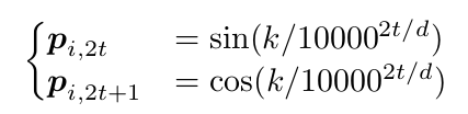
根据作者的博客文章[3],它是一种以绝对位置编码的方式实现相对位置编码的巧妙方法。怎么理解呢?我们最常见的是Transformer原始论文提出的正余弦函数:
这里的计算方式非常简单,在计算query和key时以绝对的方式之间把位置信息通过旋转向量的方式注入到向量里。计算query的时候不用考虑key,计算key的时候也不用考虑query(而其它的相对位置编码必须融合query和key一起计算)。但是”神奇”的事情发生在计算query和key的内积时,它们的内积只和它们的相对位置有关,而与绝对位置无关。用更加准确的数学语言来描述就是:
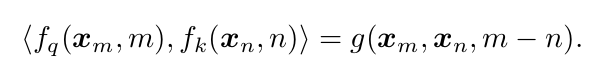
其中\(f_q(x_m,m)\)与\(f_k(x_n,n)\)是对query $x_m$以及key $x_n$进行位置编码的函数。我们用函数\(f_q(x_m,m)\)对query进行位置编码(不用考虑key),用\(f_k(x_n,n)\)对key进行编码(不用考虑query)。然后它们的内积只与(m-n)相关,而与m和n无关。
我们考虑一下query和key的位置在(1,3)和在(2,4)时,虽然计算出来的\(f_q(q,1)\)和\(f_q(q,2)\)不同,\(f_k(k,3)\)和\(f_k(k,4)\)也不相同,但是它们的内积\(<f_q(q,1),f_k(k,3)> == <f_q(q,2),f_k(k,4)>\)。
这么神奇的结果是怎么做到的呢?其实也很简单,我们以二维向量为例子。RoPE就是针对不同的位置对原始向量进行不同的旋转,比如在位置1旋转$\theta$,在位置2旋转$2\times \theta$,…。假设apple和banana的向量是$a_0$和$b_0$,假设它们的位置是1和2,那么就需要对$a_0$旋转$\theta$,对$b_0$旋转$2\times \theta$得到$a_1$和$b_1$。这个时候假设它们的夹角是$\phi$,那么它们的内积就是$\vert a \vert \vert b \vert cos \phi$。
那如果它们的位置变成了5和6,那么$a_1$和$b_1$都旋转了$4\times \theta$变成了$a_2$和$b_2$,它们的夹角还是保持不变,所以内积也不变。
TODO:画一个图。
计算公式
RoPE的计算公式为:

\(f_q(x_m,m)\)的输入是向量$x_m$和位置$m$,$W_q$是query的变换矩阵,而与m相关的是旋转矩阵$R_{\Theta,m}^d$:
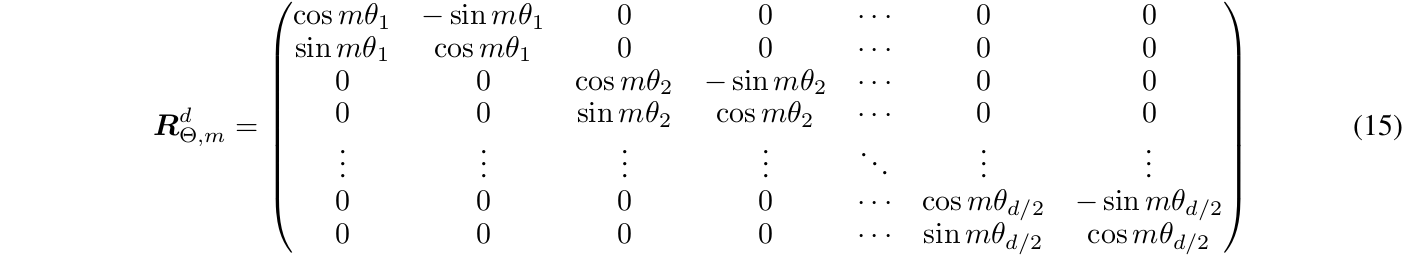
这个矩阵看起来很复杂,但是如果要计算很简单,可以把它看成$d/2 \times d/2$的分块矩阵,每个分块是一个$2 \times 2$的旋转矩阵。
如果把矩阵展开,最后的计算公式很简单:

其中$\bigotimes$表示element-wise的乘法,也就是两个向量对应位置的乘法。
RoPE的计算过程如下图所示:
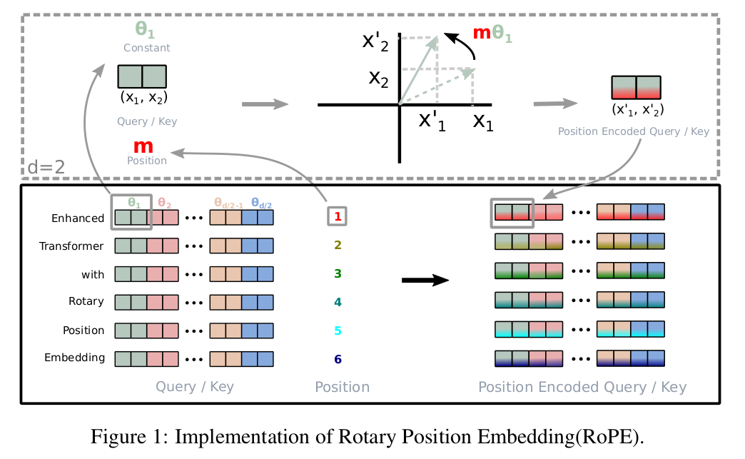
上图的例子是对输入”Enhanced Transformer with Rotary Postion Embedding”进行第一层self-attention的计算。以计算第一个token为例,如果按照原来的位置编码方法,则是用”Enhanced”的word embedding加上位置编码作为输入,然后用\(W_q\)和\(W_k\)乘得到query和key向量。而现在的方法有所不同,”Enhanced”的word embedding先乘以\(W_q\)和\(W_k\)得到query和key,这两个向量都是d维的。然后把它切分成d/2个二维向量,比如图中最前面绿色的\((x_1,x_2)\)。然后用旋转矩阵\(\begin{pmatrix} \cos m\theta_1 & - \sin m\theta_1\\ \sin m\theta_1 & \cos m\theta_1 \end{pmatrix}\)得到\((x_1',x_2')\),这里Enhanced是第一个token,所以m=1。用类似的方法可以得到query和key的第3~4,第5~6,…,第d/2-1~d/2维的向量。也就是图中右边的Position Encoded Query/Key。
代码分析
最朴素(低效)的实现
这种方法直接构造旋转矩阵$R_{\Theta,m}^d$然后做矩阵乘法,这是最简单同时也是最低效的方法。我们可以把它当成一个baseline,用它来验证其它版本的正确性。
用法
完整的代码在vanilla_rope.py,我们先看它的用法:
    torch.manual_seed(1234)
    d_model = 32
    max_seq_len = 128
    len = 50
    batch_size = 4
    pos_emb = vanilla_rope.RotaryPositionalEmbedding(d_model, max_seq_len)
    input = torch.randn(batch_size, len, d_model)
    out = pos_emb(input)
    print(out.shape)
RotaryPositionalEmbedding的构造函数需要两个必须的参数(位置参数),d_model和max_seq_len,分别代表输入向量的维度和最长序列长度。测试的输入input的shape是[4, 50, 32],我们看到输入的seq_len不用等于max_seq_len,它只需要小于等于max_seq_len就行了。
构造函数
    def __init__(self, d_model, max_seq_len, base=10000, device="cpu"):
        super().__init__()

        # Create a rotation matrix.
        self.rotation_matrix = torch.zeros(max_seq_len, d_model, d_model, device=device)

        thetas = 1.0 / (base ** (torch.arange(0, d_model, 2, device=device)
                                 .float().to(device) / d_model))

        for m in range(max_seq_len):
            m_thetas = m * thetas
            self.rotation_matrix[m].diagonal().copy_(m_thetas.cos().repeat_interleave(2))
            self.rotation_matrix[m].diagonal(offset=1)[::2].copy_(-m_thetas.sin())
            self.rotation_matrix[m].diagonal(offset=-1)[::2].copy_(m_thetas.sin())
            # matrix = torch.zeros(d_model, d_model)
            # for j in range(d_model):
            #     idx = j // 2
            #     # diagonal
            #     matrix[j, j] = torch.cos(m * thetas[idx])
            #     # superdiagonal
            #     if j < d_model - 1 and j % 2 == 0:
            #         matrix[j, j + 1] = -torch.sin(m * thetas[idx])
            #     # subdiagonal
            #     if j > 0 and j % 2 == 1:
            #         matrix[j, j - 1] = torch.sin(m * thetas[idx])
            # assert torch.equal(matrix, self.rotation_matrix[m])
__init__的主要工作就是构造旋转矩阵\(R_{\Theta,m}^d\)。
首先是计算\(\theta_i=10000^{-2(i-1)/d},i\in[1,2,...,d/2]\)。对应到代码就是:
thetas = 1.0 / (base ** (torch.arange(0, d_model, 2, device=device).float().to(device) / d_model))
公式里i是从1….d/2,所以2(i-1)是从0,2,…,d-2,这对应到代码就是range(0, dim, 2)。
接着就是按照[公式]计算。我们观察这个矩阵发现它的对角线是 [cosθ0,cosθ0,cosθ1,cosθ1,cosθ2,cosθ2……cosθd/2-1,cosθd/2-1]((代码的下标从零而不是一开始),上对角线是[-sinθ0, 0, -sinθ1, 0, …, -sinθd/2-1],下对角线是[sinθ0, 0, sinθ1, 0, …, sinθd/2-1]。用最笨的for循环方法为代码中注释掉的部分:
            # for j in range(d_model):
            #     idx = j // 2
            #     # diagonal
            #     matrix[j, j] = torch.cos(m * thetas[idx])
            #     # superdiagonal
            #     if j < d_model - 1 and j % 2 == 0:
            #         matrix[j, j + 1] = -torch.sin(m * thetas[idx])
            #     # subdiagonal
            #     if j > 0 and j % 2 == 1:
            #         matrix[j, j - 1] = torch.sin(m * thetas[idx])
但是用循环的方法是非常低效的,我们可以用更快的下标访问技巧,比如matrix[torch.arange(d), torch.arange(d)]。不过对于矩阵的对角线,pytorch的tensor提供了一个更方便的diagonal()方法,而且可以接受一个offset参数,这样除了主对角线,其它对角线也可以轻松通过offset来获取。这个方法返回的是一个view,因此我们可以用tensor的copy_方法就地修改它的内容。因为主对角线是每个cosθi连续出现两次,所以我们可以用repeat_interleave(2)来实现:
self.rotation_matrix[m].diagonal().copy_(m_thetas.cos().repeat_interleave(2))
而上对角线奇数下标是零,不需要设置,所以我们只需要设置偶数下标值:
self.rotation_matrix[m].diagonal(offset=1)[::2].copy_(-m_thetas.sin())
下对角线也是类似的。
forward方法
    def forward(self, x):
        """
        Args:
            x: A tensor of shape (batch_size, seq_len, d_model).

        Returns:
            A tensor of shape (batch_size, seq_len, d_model).
        """
        seq_len = x.shape[1]
        assert seq_len <= self.rotation_matrix.shape[0]
        m = self.rotation_matrix[:seq_len]
        out = m.unsqueeze(0) @ x.unsqueeze(-1)
        out = out.squeeze(-1)
        return out
forward的输入x的shape是[batch_size, seq_len, d_model],我们需要验证seq_len小于等于max_seq_len,然后获得旋转矩阵m。最后就是对x的最后一个维度做矩阵向量乘法从而实现向量的旋转。为了使用pytorch.matmul(@),我们需要把m从[seq_len, d_model, d_model]变成[1, seq_len, d_model, d_model],增加一个batch维度。同时把x从[batch_size, seq_len, d_model]变成[batch_size, seq_len, d_model, 1],这样pytorch.matmul就通过广播,实现最后两个维度的矩阵乘法[d_model, d_model] @ [d_model, 1] -> [d_model, 1]。返回out时要把最后一个维度squeeze掉。
Huggingface Roformer的实现
这里参考的是[5],Huggingface的文档在[6],代码在[7]。这个版本参考的是原作者在[8]的实现,原论文作者是基于keras(tensorflow)实现的。
为了更加高效以及融入整体Transformer模型里,Huggingface的实现比较复杂,核心代码在RoFormerSelfAttention的forward,其中sinusoidal_pos的计算在RoFormerSinusoidalPositionalEmbedding._init_weight。
可以使用如下的代码应用其中的RoPE部分:
    from transformers.models.roformer.modeling_roformer import (RoFormerSinusoidalPositionalEmbedding,
                                                            RoFormerSelfAttention)

    embed_positions = RoFormerSinusoidalPositionalEmbedding(max_seq_len, d_model)
    embed_positions._init_weight()
    # [sequence_length, embed_size_per_head] -> [batch_size, num_heads, sequence_length, embed_size_per_head]
    sinusoidal_pos = embed_positions(input.shape, 0)[None, None, :, :]

    layer_input = input.unsqueeze(1) # [batch, head, len, dim]

    out3, _ = RoFormerSelfAttention.apply_rotary_position_embeddings(
                            sinusoidal_pos, layer_input, layer_input
                        )
    out3 = out3.squeeze(1)
这里不做详细解读,感兴趣的读者请参考上面的链接。
Roformer简化版本
这个简化版本是根据[5]进行修改后的版本,它实现了一个RotaryPositionalEmbedding,用法和前面的简单版本完全一样。
构造函数
    def __init__(self, dim, max_position_embeddings=2048, base=10000, device="cpu"):
        super().__init__()
        self.dim = dim
        self.max_position_embeddings = max_position_embeddings
        self.base = base
        self.device = device
        #in the equation the power is negative i.e. -(2i-1), so here instead we have computed the same in denominator with +ive power
        self.inv_freq = 1.0 / (self.base ** (torch.arange(0, self.dim, 2, dtype=torch.int64).float().to(device) / self.dim))
        position_ids = torch.arange(max_position_embeddings)
        position_ids = position_ids.unsqueeze(0)
        cos, sin = self._get_cos_sin(position_ids)
        self.cos = cos
        self.sin = sin
这里的self.inv_freq就是前面实现的θ。
_get_cos_sin方法
    def _get_cos_sin(self, position_ids):
        inv_freq_expanded = self.inv_freq[None, None, :]
        # inv_freq_expanded: [1, 1, dim/2]
        position_ids_expanded = position_ids[:, :, None].float()
        # position_ids_expanded: [1, seq_len, 1]

        freqs = position_ids_expanded @ inv_freq_expanded
        # freqs: [1, seq_len, dim/2]
        cos = freqs.cos()
        # cos: [1, seq_len, dim/2]
        sin = freqs.sin()
        # sin: [1, seq_len, dim/2]
        return cos, sin
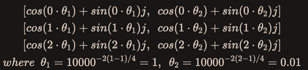
这里使用的计算公式是:
这个方法的作用是计算cos和sin,如果忽略它的第一个维度batch,它的结果等于$[cos (0\theta_1), cos (0\theta_2), …, cos (0\theta_{d/2})]$, $[cos (1\theta_1), cos (1\theta_2), …, cos (1\theta_{d/2})]$, …, \([cos ((seq\_len-1)\theta_1), cos ((seq\_len-1)\theta_2), ..., cos ((seq\_len-1)\theta_{d/2})]\)。sin也是类似的。
具体的步骤为:
- 把self.inv_freq从[dim]扩展到[1, 1, dim/2]
- 把position_ids从[1, seq_len]扩展到[1, seq_len, 1]
- freqs = position_ids_expanded @ inv_freq_expanded得到[1, seq_len, dim/2]
- 最后计算cos和sin
apply_rotary_position_embeddings静态方法
    @staticmethod
    def apply_rotary_position_embeddings(sin, cos, query_layer, key_layer):
        # sin: [1, sequence_length, embed_size_per_head//2]
        # cos: [1, sequence_length, embed_size_per_head//2]
        # query_layer: [batch_size, sequence_length, embed_size_per_head]
        # key_layer: [batch_size, sequence_length, embed_size_per_head]


        # sin [θ0,θ1,θ2......θd/2-1] -> sin_pos [θ0,θ0,θ1,θ1,θ2,θ2......θd/2-1,θd/2-1]
        sin_pos = torch.stack([sin, sin], dim=-1).reshape((sin.shape[0], sin.shape[1], sin.shape[2]*2))
        # sin_pos: [batch_size, sequence_length, embed_size_per_head]

        # cos [θ0,θ1,θ2......θd/2-1] -> cos_pos [θ0,θ0,θ1,θ1,θ2,θ2......θd/2-1,θd/2-1]
        cos_pos = torch.stack([cos, cos], dim=-1).reshape((cos.shape[0], cos.shape[1], cos.shape[2]*2))
        # cos_pos: [batch_size, sequence_length, embed_size_per_head]

        # rotate_half_query_layer [-q1,q0,-q3,q2......,-qd-1,qd-2]
        rotate_half_query_layer = torch.stack([-query_layer[..., 1::2], query_layer[..., ::2]], dim=-1).reshape_as(
            query_layer
        )
        query_layer = query_layer * cos_pos + rotate_half_query_layer * sin_pos

        # rotate_half_key_layer [-k1,k0,-k3,k2......,-kd-1,kd-2]
        rotate_half_key_layer = torch.stack([-key_layer[..., 1::2], key_layer[..., ::2]], dim=-1).reshape_as(key_layer)
        key_layer = key_layer * cos_pos + rotate_half_key_layer * sin_pos
        return query_layer, key_layer
这个函数就是对输入的query和key做RoPE,原始实现是在类RoFormerSelfAttention里,所以为了效率同时把query和key做RoPE,这样可以避免一些重复的计算。我们这里只需要抽取key(或者value)的部分就可以了,但是为了保持原来的代码,我就没有修改这个函数了,所以在调用的时候传入的key和value都是相同的输入input,这样会重复计算。另外它原来要求的输入sin和cos都是有一个batch维度的,为了调用它,我输入的sin和cos都加了一个batch维度(它们的这个维度是1,只是unsqueeze出来的为了广播用的)。
首先需要把输入的sin和cos从 [sinθ0,sinθ1,sinθ2……sinθd/2-1] -> [sinθ0,sinθ0,sinθ1,sinθ1,sinθ2,sinθ2……sinθd/2-1,sinθd/2-1],也就是把每个值都重复一下。这其实可以用我们前面用到过的repeat_interleave方法。但是这里它用的是stack来达到相同的结果(有空可以对比一些哪个效率更高):
sin_pos = torch.stack([sin, sin], dim=-1).reshape((sin.shape[0], sin.shape[1], sin.shape[2]*2))
torch.stack会多出一个维度,所以cos_pos对自己进行stack后需要reshape回去。注意stack和cat的区别:
v = torch.arange(6).reshape(2,3)
v1 = torch.stack([v, v], dim=-1)
>v1
tensor([[[0, 0],
         [1, 1],
         [2, 2]],

        [[3, 3],
         [4, 4],
         [5, 5]]])

>v1.shape
torch.Size([2, 3, 2])

>v1.reshape(2,6)
tensor([[0, 0, 1, 1, 2, 2],
        [3, 3, 4, 4, 5, 5]])
通过stack和reshape,我们可以实现类似repeat_interleave的效果。但是如果使用cat,它不会增加维度,但是不是我们想要的顺序:
>v2 = torch.cat([v, v], dim=-1)
>v2
tensor([[0, 1, 2, 0, 1, 2],
        [3, 4, 5, 3, 4, 5]])
接下来就是计算[公式],加号的左边比较好算,就是query_layer * cos_pos。后面需要先得到\((-x_2,x_1,-x_4,x_3,...,-x_{d},x_{d-1})\)。这个使用相同的stack技巧,先-query_layer[…, 1::2]得到$(-x_2, -x_4, …, -x_{d})$,query_layer[…, ::2]得到$(x_1, x_3, …, x_{d-1})$,stack后再reshape回去,就得到了交错的序列。
需要注意的是:Huggingface Roformer的实现在计算θ时用的是numpy的np.power,精度是float64并且在计算完cos和sin之后再转换成float32,而我上面的简化版本用的是torch的float(float32),所以如果对比两者的计算结果会不完全相同。
forward方法
    def forward(self, x):
        """
        Args:
            x: A tensor of shape (batch_size, seq_len, d_model).

        Returns:
            A tensor of shape (batch_size, seq_len, d_model).
        """
        batch_size, seq_len = x.shape[:2]
        assert seq_len <= self.cos.shape[1]
        cos, sin = self.cos[:,:seq_len], self.sin[:,:seq_len]
        out, _ = RotaryPositionalEmbedding.apply_rotary_position_embeddings(
                        sin, cos, x, x
                    )

        return out
huggingface Llama实现
这个版本的实现和Roformer的基本类似,完整的代码可以参考这里。
它和Roformer的区别在于:Roformer的实现是严格按照公式来的。对于cos部分,排列顺序是[cosθ0,cosθ0,cosθ1,cosθ1,cosθ2,cosθ2……cosθd/2-1,cosθd/2-1],对应的x是[x0,x1,x2,x3,….,xd-2,xd-1]。而对于cos,对应的x是[-x1,x0,-x3,x2,….]。
而huggingface Llama的实现如下图:
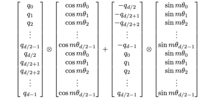
它cos和x排列顺序是
[cosθ0,cosθ1,cosθ2,...cosθd/2-1,  ....         cosθ0,cosθ1 ,cosθ2, .... cosθd/2-1]
[q0   ,q1   ,q2   ,...qd/2-1   ,  ....         qd/2 ,qd/2+1,qd/2+2 .... qd-1     ]
如果我们把q0,…qd/2-1对应x的偶数下标部分,qd/2,…,qd-1对应x的奇数下标部分:
[cosθ0,cosθ1,cosθ2,...cosθd/2-1,  ....         cosθ0,cosθ1 ,cosθ2, .... cosθd/2-1]
[q0   ,q1   ,q2   ,...qd/2-1   ,  ....         qd/2 ,qd/2+1,qd/2+2 .... qd-1     ]
[x0   ,x2,  ,x4   ,...xd-2     ,  ....         x1   ,x3    ,x5     .... xd-1     ]
把它换一下顺序就会原来的公式一样了(对比一下第一行和第三行):
[cosθ0,cosθ0,cosθ1,cosθ1 ,cosθ2,cosθ2,...cosθd/2-1,  ....          .... cosθd/2-1]
[q0   ,qd/2 ,q1   ,qd/2+1,q2   ,qd/2+2 ...qd/2-1   ,  ....         .... qd-1     ]
[x0   ,x1   ,x2,  ,x3    ,x4   ,x5     ...xd-2     ,  ....         .... xd-1     ]
为什么会搞成这样呢?这是因为huggingface的输入就是这样排布的(我也没有搞明白它为什么搞成了这样)。所以这也是为什么[10]和[11]里提到的从meta llama格式转换成huggingface llama时需要permute:
 def permute(w, n_heads=n_heads, dim1=dim, dim2=dim):
     return w.view(n_heads, dim1 // n_heads // 2, 2, dim2).transpose(1, 2).reshape(dim1, dim2)
现在我们假设输入的q和之前的x有这样奇怪的对应关系,那么我们再看sin的部分,它需要的是:
[sinθ0,  sinθ1      ,sinθ2,... ,sinθd/2-1,  ....         sinθ0,sinθ1 ,sinθ2, .... sinθd/2-1]
[-qd/2   ,-qd/2+1   ,qd/2+2,...,qd-1     ,  ....         q0   ,q1    ,q2   , .... qd/2-1   ]
这个排布通过函数rotate_half来实现:
def rotate_half(x):
    """Rotates half the hidden dims of the input."""
    x1 = x[..., : x.shape[-1] // 2]
    x2 = x[..., x.shape[-1] // 2 :]
    return torch.cat((-x2, x1), dim=-1)
比如一个例子:
>x=torch.arange(8)

>x
tensor([0, 1, 2, 3, 4, 5, 6, 7])

>rotate_half(x)
tensor([-4, -5, -6, -7,  0,  1,  2,  3])
Meta Llama的实现
这部分内容主要参考[An In-depth exploration of Rotary Position Embedding (RoPE)],它参考的是Llama的官方代码。
这个实现比较有意思的是通过复数乘法来实现旋转矩阵乘法相同的功能。这两种计算方法完全相同,因为不管是矩阵向量乘法还是复数乘法,最后都是数字的乘法和加分!这样的实现相比朴素的矩阵乘法更加高效,但是又不需要前面方法的各种下标tricks。
在介绍它的代码之前,我们先回顾一下复指数和二维旋转矩阵的关系。
复指数和二维旋转
关于复指数和二维旋转,这个视频讲的很易懂。我这里列举一下主要结论。
对于二维平面的向量$(a, b)$,把它逆时针旋转$\theta$,得到新的向量是$(a’, b’)$。计算方法为:
\[\begin{pmatrix} a' \\ b' \end{pmatrix} = \begin{pmatrix} \cos \theta & -\sin \theta \\ \sin \theta & \cos \theta \end{pmatrix} \begin{pmatrix} a \\ b \end{pmatrix} = \begin{pmatrix} a \cos \theta - b \sin \theta \\ a \sin \theta + b \cos \theta \end{pmatrix}\]如果我们把旋转矩阵替换成复数$\cos \theta + i \sin \theta$,并且把向量看成复平面的复数$a + ib, a’ + ib’$,那么有:
\[a' + ib' = (a + ib)(\cos \theta + i \sin \theta)\]用复数乘法公式把它展开(把i看成一个符号并且记得$i^2=-1$就行了):
\[(a + ib)(\cos \theta + i \sin \theta) = (a \cos \theta + i^2 b \sin \theta) + (a \sin \theta + b \cos \theta)i = (a \cos \theta - b \sin \theta) + (a \sin \theta + b \cos \theta)i\]两个复数相等的条件是实部和虚部都相等,所以就可以得到:
\[a' = a \cos \theta - b \sin \theta \\ b' = a \sin \theta + b \cos \theta\]把它写成矩阵乘以向量的形式(不会的话可以反过来用下面的式子做一下[2x2]x2的矩阵向量乘法来验证):
\[\begin{pmatrix} a' \\ b' \end{pmatrix} = \begin{pmatrix} \cos \theta & -\sin \theta \\ \sin \theta & \cos \theta \end{pmatrix} \begin{pmatrix} a \\ b \end{pmatrix}\]所以对一个二维向量$v$做逆时针$\theta$的旋转,等价于把这个二维向量看成复数,然后乘以$\cos \theta + i \sin \theta$。而根据欧拉公式$\cos \theta + i \sin \theta = e^{i\theta}$,也可以写成$v’ = ve^{i\theta}$。忘了欧拉公式的也不要被吓到了,这只是一种记号而已。我们在下面实际的计算中根本不需要用到欧拉公式,只需要知道复数的乘法公式(其实也不需要自己算)就可以实现等价的旋转矩阵乘以向量了。
构造函数
    def __init__(self, d_model, max_seq_len, base=10000.0, device="cpu"):
        self.freqs_cis = RotaryPositionalEmbedding.precompute_freqs_cis(
            d_model, max_seq_len, base
        )
初始化就是构造旋转矩阵的复数形式,具体实现在下面的precompute_freqs_cis。
precompute_freqs_cis函数
    @staticmethod
    def precompute_freqs_cis(dim: int, end: int, theta: float = 10000.0):
        """
        Precompute the frequency tensor for complex exponentials (cis) with given dimensions.

        This function calculates a frequency tensor with complex exponentials using the given dimension 'dim'
        and the end index 'end'. The 'theta' parameter scales the frequencies.
        The returned tensor contains complex values in complex64 data type.

        Args:
            dim (int): Dimension of the frequency tensor.
            end (int): End index for precomputing frequencies.
            theta (float, optional): Scaling factor for frequency computation. Defaults to 10000.0.

        Returns:
            torch.Tensor: Precomputed frequency tensor with complex exponentials.


        """
        # Each group contains two components of an embedding,
        # calculate the corresponding rotation angle theta_i for each group.
        freqs = 1.0 / (theta ** (torch.arange(0, dim, 2)[: (dim // 2)].float() / dim))
        # Generate token sequence index m = [0, 1, ..., sequence_length - 1]
        t = torch.arange(end, device=freqs.device)  # type: ignore
        # Calculate m * theta_i
        freqs = torch.outer(t, freqs).float()  # type: ignore
        freqs_cis = torch.polar(torch.ones_like(freqs), freqs)  # complex64
        return freqs_cis
这段代码freqs的计算和前面完全一样,它的shape是[max_seq_len, dim],每i列表示[iθ0, iθ1, …, iθdim/2-1]。和前面稍微有一点点区别在于用的是两个向量的外积(torch.outer),它的效果和矩阵乘法(max_seq_len, 1) x (1, dim)是一样的。
和之前不一样的是这里没有用freqs来计算$\sin, \cos$。而是使用torch.polar来生成复数。这里我们先看一下torch.polar这个函数。
根据官方文档,这个函数的签名是:
torch.polar(abs, angle, *, out=None) → Tensor
这个函数实现的功能是:out=abs⋅cos(angle)+abs⋅sin(angle)⋅j
也就是说,输入是复数的模(长度)向量和辐角,返回这个复数的笛卡尔坐标。我们看一个例子:
>>> import numpy as np
>>> abs = torch.tensor([1, 2], dtype=torch.float64)
>>> angle = torch.tensor([np.pi / 2, 5 * np.pi / 4], dtype=torch.float64)
>>> z = torch.polar(abs, angle)
>>> z
tensor([(0.0000+1.0000j), (-1.4142-1.4142j)], dtype=torch.complex128)
这里输入了两个复数,一个模是1,辐角是90°;另一个长度2,辐角是225°。我们看到返回的是两个复数:0+1j, -1.4142-1.4142j。 这里输入的模和辐角是float64,返回的是complex128。complex128可以认为是两个float64拼接起来,一个float代表复数的实部,另一个代表虚部。而且实际在内存中的存储也是这样的,所以后面我们可以把一个复数view成两个实数,也可以把两个实数view成一个复数。
明白了torch.polar,我们回到前面的代码:
freqs_cis = torch.polar(torch.ones_like(freqs), freqs)
我们前面的freqs是角度,而我们的旋转矩阵对应的复数的模都1,所以它用的是torch.ones_like。由于我们输入的freqs的shape是[max_seq_len, dim/2],dtype是float32,所以返回的freqs_cis的shape也是[max_seq_len, dim/2],dtype是complex64。
我们用一个简单的例子来具体看一下这个计算过程和结果,我们假设dim=4,max_seq_len=3,那么计算的过程为:
结果为:
tensor([[ 1.0000+0.0000j,  1.0000+0.0000j],
        [ 0.5403+0.8415j,  0.9999+0.0100j],
        [-0.4161+0.9093j,  0.9998+0.0200j]])
看起来和之前不一样,但是其实torch.polar同样计算了 sin[iθ0, iθ1, …, iθdim/2-1]和cos[iθ0, iθ1, …, iθdim/2-1],只不过存放的位置合并到一个复数里而已。后面我们会看到怎么用复数的乘法完成同样的旋转矩阵的运算。
forward方法
    def forward(self, x):
        """
        Args:
            x: A tensor of shape (batch_size, seq_len, d_model).

        Returns:
            A tensor of shape (batch_size, seq_len, d_model).
        """
        bsz, seqlen, _ = x.shape
        xq = x.view(bsz, seqlen, 1, -1)
        xq, _ = RotaryPositionalEmbedding.apply_rotary_emb(xq, xq, freqs_cis=self.freqs_cis[:seqlen])

        return xq.squeeze(2)
forward把输入x(比如[4,3,4]的tensor)reshape成[4,3,1,4],多出来的维度是MHA的多个head。我们这里假设只有一个head。然后就是调用apply_rotary_emb函数进行计算。
apply_rotary_emb函数
    @staticmethod
    def apply_rotary_emb(
        xq: torch.Tensor,
        xk: torch.Tensor,
        freqs_cis: torch.Tensor,
    ) -> Tuple[torch.Tensor, torch.Tensor]:
        """
        Apply rotary embeddings to input tensors using the given frequency tensor.

        This function applies rotary embeddings to the given query 'xq' and key 'xk' tensors using the provided
        frequency tensor 'freqs_cis'. The input tensors are reshaped as complex numbers, and the frequency tensor
        is reshaped for broadcasting compatibility. The resulting tensors contain rotary embeddings and are
        returned as real tensors.

        Args:
            xq (torch.Tensor): Query tensor to apply rotary embeddings.
            xk (torch.Tensor): Key tensor to apply rotary embeddings.
            freqs_cis (torch.Tensor): Precomputed frequency tensor for complex exponentials.

        Returns:
            Tuple[torch.Tensor, torch.Tensor]: Tuple of modified query tensor and key tensor with rotary embeddings.

        """
        # Reshape and convert xq and xk to complex number
        xq_ = torch.view_as_complex(xq.float().reshape(*xq.shape[:-1], -1, 2))
        xk_ = torch.view_as_complex(xk.float().reshape(*xk.shape[:-1], -1, 2))
        freqs_cis = RotaryPositionalEmbedding.reshape_for_broadcast(freqs_cis, xq_)
        # Apply rotation operation, and then convert the result back to real numbers.
        xq_out = torch.view_as_real(xq_ * freqs_cis).flatten(3)
        xk_out = torch.view_as_real(xk_ * freqs_cis).flatten(3)
        return xq_out.type_as(xq), xk_out.type_as(xk)
我们首先看第一个语句:
xq_ = torch.view_as_complex(xq.float().reshape(*xq.shape[:-1], -1, 2))
输入xq的shape是[4,3,1,4],代表[batch,len,num_head,dim],我们需要把两个x变成一个复数,所以reshape成[4,3,1,-1,2],也就是[4,3,1,4/2,2]=[4,3,1,2,2]。
而torch.view_as_complex把最后一个维度的两个实数看成一个复数,最终的xq_就是[4,3,1,2],代表[batch,len,num_head,dim/2]。
freqs_cis的shape是[3,2],代表[max_len,dim/2],为了能够进行复数乘法需要调用reshape_for_broadcast。调用之后的freqs_cis的shape是[1,3,1,2],代表[batch,len,num_head,dim/2]。然后是最关键的语句:
xq_out = torch.view_as_real(xq_ * freqs_cis).flatten(3)
首先是复数乘法xq_ * freqs_cis,我们以第一个复数为例:
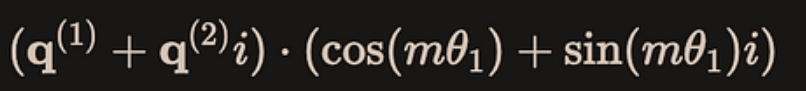
query里的前两个数是$q^{(1)}, q^{(2)}$,前面的view_as_complex已经把它变成了$q^{(1)} + q^{(2)}i$,类似的,freqs_cis的第一个复数是$\cos (m\theta_1) + \sin (m\theta_1) i$,然后两个复数乘法的结果通过view_as_real又拆分成实部和虚部就是:

而这个结果就是下图大矩阵乘法中红色的两个分块矩阵的乘法:
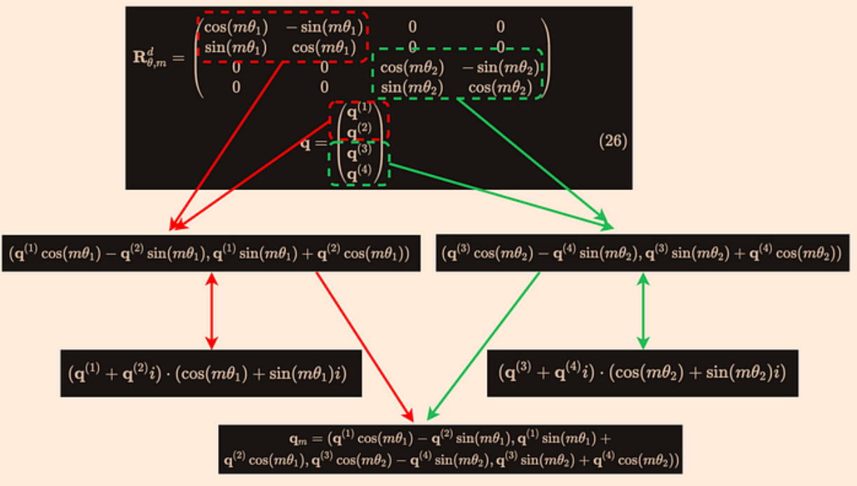
这样得到的结果的shape是[4,3,1,2,2],代表[batch, len, num_head, dim/2, 2],最后我们用flatten(3)把它reshape个[4,3,1,4]。
reshape_for_broadcast函数
    @staticmethod
    def reshape_for_broadcast(freqs_cis: torch.Tensor, x: torch.Tensor):
        """
        Reshape frequency tensor for broadcasting it with another tensor.

        This function reshapes the frequency tensor to have the same shape as the target tensor 'x'
        for the purpose of broadcasting the frequency tensor during element-wise operations.

        Args:
            freqs_cis (torch.Tensor): Frequency tensor to be reshaped.
            x (torch.Tensor): Target tensor for broadcasting compatibility.

        Returns:
            torch.Tensor: Reshaped frequency tensor.

        Raises:
            AssertionError: If the frequency tensor doesn't match the expected shape.
            AssertionError: If the target tensor 'x' doesn't have the expected number of dimensions.
        """
        ndim = x.ndim
        assert 0 <= 1 < ndim
        assert freqs_cis.shape == (x.shape[1], x.shape[-1])
        shape = [d if i == 1 or i == ndim - 1 else 1 for i, d in enumerate(x.shape)]
        return freqs_cis.view(*shape)
我没明白 assert 0 <= 1 < ndim,为什么有个永远True的 0 <= 1。这个函数就是检查freqs_cis.shape匹配x.shape[1]和x.shape[-1],然后把其它的维度设置成和x相同。
总结
在这个版本的实现里,通过torch.polar实现了cosθ和sinθ的计算,而且对于每个位置m,每行排列成[cos(mθ1)+sin(mθ1)i, cos(mθ2)+sin(mθ2)i, …, cos(mθd/2)+sin(mθd/2)i]的形式。而输入的q也是排列成[q1+q2i,q3+q4i,….,q(d/2-1)+q(d/2)i],最后通过复数的乘法实现了等价的旋转矩阵计算。它的计算量和前面Roformer完全相同,但是不需要我们考虑各种下标的tricks。这种实现还是挺巧妙的!
其它版本
比如[这个网页]排版非常好,代码和注释左右对照,强烈建议关注labml.ai Deep Learning Paper Implementations,里面有各种论文的代码实现。
此外还有torchtune的RoPE实现。
它们的代码都大同小异,因为相对来说用的比较少,我这里就不分析了。
参考文献
- [1] RoFormer: Enhanced Transformer with Rotary Position Embedding
- [2] RoPE论文解读
-
[4] Rotary Positional Embeddings: A Detailed Look and Comprehensive Understanding
-
[5] Rotary Positional Embedding(RoPE): Motivation and Code Implementation
-
[9] An In-depth exploration of Rotary Position Embedding (RoPE)
-
[11] [LLaMA] Rotary positional embedding differs with official implementation
- [12] RoPE代码公式对照版
- 显示Disqus评论(需要科学上网)